Uncertainty analysis of GiveWell's cost-effectiveness analysis
GiveWell produces cost-effectiveness models of its top charities. These models take as inputs many uncertain parameters. Instead of representing those uncertain parameters with point estimates—as the cost-effectiveness analysis spreadsheet does—we can (should) represent them with probability distributions. Feeding probability distributions into the models allows us to output explicit probability distributions on the cost-effectiveness of each charity.
Contents
GiveWell’s cost-effectiveness analysis
GiveWell, an in-depth charity evaluator, makes their detailed spreadsheets models available for public review. These spreadsheets estimate the value per dollar of donations to their 8 top charities: GiveDirectly, Deworm the World, Schistosomiasis Control Initiative, Sightsavers, Against Malaria Foundation, Malaria Consortium, Helen Keller International, and the END Fund. For each charity, a model is constructed taking input values to an estimated value per dollar of donation to that charity. The inputs to these models vary from parameters like “malaria prevalence in areas where AMF operates” to “value assigned to averting the death of an individual under 5”.
Helpfully, GiveWell isolates the input parameters it deems as most uncertain. These can be found in the “User inputs” and “Moral weights” tabs of their spreadsheet. Outsiders interested in the top charities can reuse GiveWell’s model but supply their own perspective by adjusting the values of the parameters in these tabs.
For example, if I go to the “Moral weights” tab and run the calculation with a 0.1 value for doubling consumption for one person for one year—instead of the default value of 1—I see the effect of this modification on the final results: deworming charities look much less effective since their primary effect is on income.
Uncertain inputs
GiveWell provides the ability to adjust these input parameters and observe altered output because the inputs are fundamentally uncertain. But our uncertainty means that picking any particular value as input for the calculation misrepresents our state of knowledge. From a subjective Bayesian point of view, the best way to represent our state of knowledge on the input parameters is with a probability distribution over the values the parameter could take. For example, I could say that a negative value for increasing consumption seems very improbable to me but that a wide range of positive values seem about equally plausible. Once we specify a probability distribution, we can feed these distributions into the model and, in principle, we’ll end up with a probability distribution over our results. This probability distribution on the results helps us understand the uncertainty contained in our estimates and how literally we should take them.
Is this really necessary?
Perhaps that sounds complicated. How are we supposed to multiply, add and otherwise manipulate arbitrary probability distributions in the way our models require? Can we somehow reduce our uncertain beliefs about the input parameters to point estimates and run the calculation on those? One candidate is to take the single most likely value of each input and using that value in our calculations. This is the approach the current cost-effectiveness analysis takes (assuming you provide input values selected in this way). Unfortunately, the output of running the model on these inputs is necessarily a point value and gives no information about the uncertainty of the results. Because the results are probably highly uncertain, losing this information and being unable to talk about the uncertainty of the results is a major loss. A second possibility is to take lower bounds on the input parameters and run the calculation on these values, and to take the upper bounds on the input parameters and run the calculation on these values. This will produce two bounding values on our results, but it’s hard to give them a useful meaning. If the lower and upper bounds on our inputs describe, for example, a 95% confidence interval, the lower and upper bounds on the result don’t (usually) describe a 95% confidence interval.
Computers are nice
If we had to proceed analytically, working with probability distributions throughout, the model would indeed be troublesome and we might have to settle for one of the above approaches. But we live in the future. We can use computers and Monte Carlo methods to numerically approximate the results of working with probability distributions while leaving our models clean and unconcerned with these probabilistic details. Guesstimate is a tool that works along these lines and bills itself as “A spreadsheet for things that aren’t certain”.
Analysis
We have the beginnings of a plan then. We can implement GiveWell’s cost-effectiveness models in a Monte Carlo framework (PyMC3 in this case), specify probability distributions over the input parameters, and finally run the calculation and look at the uncertainty that’s been propagated to the results.
Model
The Python source code implementing GiveWell’s models can be found on GitHub1. The core models can be found in cash.py, nets.py, smc.py, worms.py and vas.py.
Inputs
For the purposes of the uncertainty analysis that follows, it doesn’t make much sense to infect the results with my own idiosyncratic views on the appropriate value of the input parameters. Instead, what I have done is uniformly taken GiveWell’s best guess and added and subtracted 20%. These upper and lower bounds then become the 90% confidence interval of a log-normal distribution2. For example, if GiveWell’s best guess for a parameter is 0.1, I used a log-normal with a 90% CI from 0.08 to 0.12.
While this approach screens off my influence it also means that the results of the analysis will primarily tell us about the structure of the computation rather than informing us about the world. Fortunately, there’s a remedy for this problem too. I have set up a Jupyter notebook3 with the all the input parameters to the calculation which you can manipulate and rerun the analysis. That is, if you think the moral weight given to increasing consumption ought to range from 0.8 to 1.5 instead of 0.8 to 1.2, you can make that edit and see the corresponding results. Making these modifications is essential for a realistic analysis because we are not, in fact, equally uncertain about every input parameter.
It’s also worth noting that I have considerably expanded the set of input parameters receiving special scrutiny. The GiveWell cost-effectiveness analysis is (with good reason—it keeps things manageable for outside users) fairly conservative about which parameters it highlights as eligible for user manipulation. In this analysis, I include any input parameter which is not tautologically certain. For example, “Reduction in malaria incidence for children under 5 (from Lengeler 2004 meta-analysis)” shows up in the analysis which follows but is not highlighted in GiveWell’s “User inputs” or “Moral weights” tab. Even though we don’t have much information with which to second guess the meta-analysis, the value it reports is still uncertain and our calculation ought to reflect that.
Results
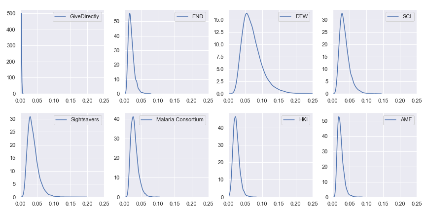
Finally, we get to the part that you actually care about, dear reader: the results. Given input parameters which are each distributed log-normally with a 90% confidence interval spanning ±20% of GiveWell’s best estimate, here are the resulting uncertainties in the cost-effectiveness estimates:

For reference, here are the point estimates of value per dollar using GiveWell’s values for the charities:
| Charity | Value per dollar |
|---|---|
| GiveDirectly | 0.0038 |
| The END Fund | 0.0222 |
| Deworm the World | 0.0738 |
| Schistosomiasis Control Initiative | 0.0378 |
| Sightsavers | 0.0394 |
| Malaria Consortium | 0.0326 |
| Helen Keller International | 0.0223 |
| Against Malaria Foundation | 0.0247 |
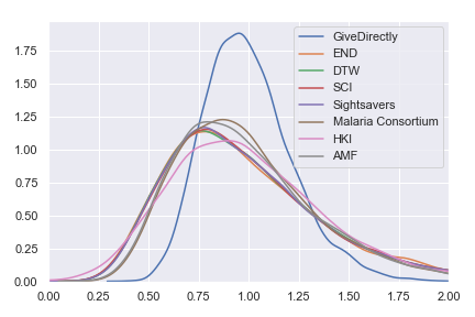
I’ve also plotted a version in which the results are normalized—I divided the results for each charity by that charity’s expected value per dollar. Instead of showing the probability distribution on the value per dollar for each charity, this normalized version shows the probability distribution on the percentage of that charity’s expected value that it achieves. This version of the plot abstracts from the actual value per dollar and emphasizes the spread of uncertainty. It also reëmphasizes the earlier point that—because we use the same spread of uncertainty for each input parameter—the current results are telling us more about the structure of the model than about the world. For real results, go try the Jupyter notebook!

Conclusions
Our preliminary conclusion is that all of GiveWell’s top charities cost-effectiveness estimates have similar uncertainty with GiveDirectly being a bit more certain than the rest. However, this is mostly an artifact of pretending that we are exactly equally uncertain about each input parameter.
Unfortunately, the code implements the 2019 V4 cost-effectiveness analysis instead of the most recent V5 because I just worked off the V4 tab I’d had lurking in my browser for months and didn’t think to check for a new version until too late. I also deviated from the spreadsheet in one place because I think there’s an error (Update: The error will be fixed in GiveWell’s next publically-released version).↩︎
Log-normal strikes me as a reasonable default distribution for this task: because it’s support is (0, +∞) which fits many of our parameters well (they’re all positive but some are actually bounded above by 1); and because “A log-normal process is the statistical realization of the multiplicative product of many independent random variables” which also seems reasonable here.↩︎
When you follow the link, you should see a Jupyter notebook with three “cells”. The first is a preamble setting things up. The second has all the parameters with lower and upper bounds. This is the part you want to edit. Once you’ve edited it, find and click “Runtime > Run all” in the menu. You should eventually see the notebook produce a serious of plots.↩︎