Taking social choice seriously: An alternative approach to reward modeling in RLHF

RLHF

Reinforcement learning from human feedback (RLHF)¹ is a by-now conventional technique for making pre-trained² language models responsive to a variety of human preferences.

The standard RLHF setup involves (this is not meant to be a comprehensive description):

1. Collecting human preference data about pairs (or more) of language model outputs.
2. Training a reward model on this preference data according to a Bradley-Terry model (There have been many recent papers which adjust this in some way. But I’ve not seen any that obsolete this post.). This model produces a scalar reward for a language model completion—in the context of a prompt—that somehow reflects the rater data.
3. Aligning the language model to the reward model.

In everything that follows, we’re focused exclusively on step 2.

Social choice theory

Social choice theory³ is a rich body of theory on how to aggregate individual preferences into collective, social decisions. Think voting systems. For example, in a presidential election, each ballot expresses some aspect of an individual’s preferences over the candidates. And the voting system aggregates those ballots into a single decision about the next president. Arrow’s impossibility theorem is assuredly the most famous result in social choice theory, if that jogs your memory.

Vanilla RLHF as social choice

As⁴ we outlined above, for a given prompt, the RLHF reward modeling step starts with:

• A set of choices—language model outputs for the prompt
• A set of individuals—raters
• Preference orders over these choices for these indivduals

And produces:

• A reward model which represents a singular preference order over the choices

But this is precisely the social choice problem! We have transformed a set of individual preference orders into a single, social preference order. We can then think of the reward modeling process as running a series of such preference aggregations—one voting contest per prompt.

Making the implicit explicit

RLHF⁵ is usally not framed quite so explicitly in these terms, but I claim that doing so brings clarity and highlights issues with the vanilla approach. The loss function specified in Training language models to follow instructions with human feedback is:

\[ \text{loss}(\theta) = -\frac{1}{\left(\frac{K}{2}\right)} \mathbb{E}_{(x,y_w,y_l)\sim D}\left[ \log \left( \sigma (r_\theta (x,y_w) - r_\theta (x,y_l))\right)\right] \]

“where \(r_\theta(x,y)\) is the scalar output of the reward model for prompt x and completion y with parameters \(\theta\), \(y_w\) is the preferred completion out of the pair of \(y_w\) and \(y_l\), and \(D\) is the dataset of human comparisons.”

We can think of this loss function as implementing a random ballot preference aggregation rule wherein the preference of the arbitrary rater is taken as the social preference the reward model should learn. If we had complete rater data (i.e. each rater had rated every completion)⁶, a sequence of updates according to this loss function across many epochs would converge to the Borda count outcome. (In Borda count, each voter submits a ranked list of the choices and the choices are assigned scores based on this ranking—e.g. for a contest with 3 choices, the choice in 3rd place gets 0 points, the choice in 2nd place gets 1 point, and the choice in 1st place gets 2 points. Points for each candidate are summed across all voters and the social preference order is the list of choices sorted by these sums.)

Normative analysis

Social choice criteria

With⁷ all that in mind, how do we feel about Borda count as a preference aggregation rule? The social choice literature has already established a number of criteria according to which we can evaluate preference aggregation rules. This table is fun to peruse on a rainy afternoon. Some criteria which we might want a preference aggregation rule to satisfy include:

Majority

“if only one candidate is ranked first by a majority (more than 50%) of voters, then that candidate must win.”

Condorcet winner

If there’s a candidate that would beat all other candidates in pairwise contests, that candidate should win.

Independence of irrelevant alternatives

If A would beat B without C present in the contest, then A should still beat B when C is present⁸. The highly quotable Sydney Morgenbesser illustrated it thus: “Morgenbesser, ordering dessert, is told by a waitress that he can choose between blueberry or apple pie. He orders apple. Soon the waitress comes back and explains cherry pie is also an option. Morgenbesser replies ‘In that case, I’ll have blueberry.’”

Borda count satisfies none of these criteria. This presentation is a little unfair because Arrow famously (famous to a certain kind of nerd) demonstrated that no preference aggregation rule (in a certain setting) can satisfy all intuitively desirable criteria. But it still might be the case that we’d prefer our increasingly important AI systems to be guided by a deliberately chosen preference aggregation rule with a careful consideration of the trade-offs involved rather than just YOLOing off into the unknown with the first thing we happened to accidentally implement.

Worst-case scenarios

That’s⁹ theoretically interesting but, if we can’t get a perfect preference aggregation rule anyway, maybe Borda count’s infelicities don’t matter? Does a social choice perspective just help us futz around with details? If we’re truly doom-pilled, maybe the most important thing is ensuring that our preference aggregation rule doesn’t introduce any additional routes to catastrophe. It turns out social-choice-induced catastrophe is on the table!

It’s perhaps reasonable to think of individuals as having underlying cardinal utility functions and that the preference orders used in a voting system are imperfect reflections of these utility functions. In this setting, we can sensibly ask: “What sorts of social utility (i.e. the mean of individual utilities) are produced by our preference aggregation rule?”. It turns out that many preference aggregation rules, including Borda count, produce unbounded distortion! In other words, the outcome selected by the preference aggregation rule can have an arbitrarily large negative utility.

We can see the basic intuition behind this result with an example. Suppose we have a population with utilities over choices like this:

1. A: 1.0, B: 0.9999: C: 0.9998, D: 0.9997: E: 0.9996
2. E: 1.0, A: -0.9997, B: -0.9998, C: -0.9999, D: -1.0

If \(20 + \epsilon\%\) of the population has the first set of utilities and \(80 - \epsilon\%\) of the population has the second set of utilities, then Borda count will select A as the social choice. But the utility of this choice is approximately \(0.2 \cdot 1 + 0.8 \cdot -1 = -0.6\) while the social utility maximizing choice is E with an approximate utility of 1.

So a poorly chosen preference aggregation rule can lead to social outcomes which are quite bad indeed.

Strategic voting

A related¹⁰ concern higlighted by the social choice perspective is the possibility of strategic voting. One of the central concerns of social choice theory (and especially mechanism design) is accounting for the fact that nothing compels an individual to simply honestly report their preferences. Many voters are strategic actors who will instead report the preferences which are most likely to help them achieve their preferred outcomes.

I think this concern also applies to raters in an RLHF setup. I certainly imagine that I would feel the temptation to adjust my ratings based on strategic concerns were I a rater. So we also need to make sure our RLHF setup is robust to strategic behavior and I’ve seen little consideration of this angle.

(And, to make the connection explicit, strategic behavior accentuates the possibility of utilitarian distortions. Without strategic behavior, we can fall back to the idea “Well, the outcome chosen can’t be that perverse because at least some human wanted it.” But with strategic behavior in the mix, this defense no longer holds.)

Social choice RLHF

Suppose¹¹ we take all that analysis seriously and regard vanilla RHLF as having important limitations. Can we do anything about it? Did we come to create or only destroy? Create! We can adjust the reward model in the RLHF setup to more closely mimic the social choice formalism. The key is that, instead of a singular reward model, we train two distinct reward models. We have an individual reward model which learns to represent the various sorts of preferences individuals have and a social reward model which learns social preferences. We link the two via a preference aggregation rule of our choosing. In slightly more detail, the process looks like:

1. Train a stochastic “individual reward model” on rater data. This model learns to both: represent the different kinds of preferences individuals can have in a sample-able latent space; and provide a scalar output representing reward for a completion given a preference representation from this latent space.
2. Embed all raters in the latent space and then do ex post density estimation¹² (by e.g. fitting a Gaussian mixture model).
3. Sample from the latent space via the estimated distribution to generate a population of simulated individual voters.
4. Have a language model generate completions for a series of prompts. (Or just reuse the prompt and completion set presented to raters. But you don’t have to do so. All the rater info should be embodied in the individual reward model at this point so we are untethered from the rater prompts and completions.)
5. For each contest (i.e. a set of completions for a single prompt), we use the individual reward model to produce a preference order¹³ over the completions for each simulated voter.
6. Run the preference aggregation rule of our choosing over these preference orders to produce a social preference order.
7. Train a social reward model on this social preference order. This is essentially the same as the original reward model training in vanilla RLHF but with a different preference order as input.

(If you’d prefer a less ambiguous description, the full code accompanying this post is available in this repository.)

We can see that this approach is a strict generalization of the vanilla RLHF reward model. If the preference aggregration rule we choose in step 6 is a random ballot rule, then the social reward model will (roughly, there are some other angles we’ll cover later) learn the same preference order as the vanilla RLHF reward model. But we’re no longer forced into this choice—we can choose whichever preference aggregation rule we want in step 6 since we have the social choice prerequisites at hand: a complete set of ordinal preferences for all individuals¹⁴.

Individual reward model

The¹⁵ trickiest new element in the above outline is the individual reward model. We show the essential architecture during training in the figure below. Note that round-corned boxes represent data sources and sinks, parallelograms represent fixed operations, and square-cornered boxes represent learned operations.

The input is a complete set of data for a single rater—all N prompts they have rated completions for and all M completions (in ranked order) for each of those prompts. This allows the model to learn a comprehensive representation of the rater’s preferences across a variety of contexts.

These nested sequences are flattened into a single sequence with appropriate position info added to track the relative order of the completions. The encoder compresses this variable length sequence into a single fixed length representation (in our case, this is done by a transformer decoder which cross-attends to the sequence as the keys and values and uses a single-element dummy sequence of the appropriate width as the query). This fixed length representation as used as the mean for a sampler block which produces an output with an isotropic Gaussian distribution around this mean via the reparameterization trick. At this point, the preferences should be represented in a smooth latent space similar to the latent bottleneck in a variational autoencoder. This latent preference representation is then decoded into a form that’s usable by the reward block. The reward block produces a scalar reward when given a completion and, unlike the vanilla reward model, an additional preference representation to condition on. The reward block is vmaped to produce a reward for each completion for each prompt. The reward scores for each completion within a prompt are passed into list MLE loss function to encourage the right relative rewards across the whole sequence.

If you’d rather just look at the code, see the architecture module.

At a higher level, we can see that this is also a strict generalization of the vanilla RLHF reward model—instead of producing a scalar reward based on just the completion, the final reward block also gets to condition on a representation of the individual’s preferences. If we force the sampler to always emit a constant, dummy preference representation, we recover the vanilla RLHF reward model which tries to learn the ordering that best simultaneously satisfies all raters.

There’s also a strong similarity to VAEs. The primary difference is that, instead of reconstructing the full input, the model learns to reconstruct just the ordering of the completions. We also don’t necessarily have any strong prior beliefs about the appropriate dimensionality of the latent space (We have, alas, not yet much characterized the manifold of human desire.). So we can’t rely on reduced dimensionality to force abstraction or compression. Instead we have to do some careful masking on the inputs and outputs to ensure that the model learns a useful, abstract representation of preferences. The details are covered in the appendix.

Does this all work?

Yes¹⁶. I’ve tested this architecture on a number of synthetic, small rater datasets. The social reward model can faithfully learn both Borda count social preferences and the social preferences specified by other aggregation rules. More detailed evidence that the learned latent space of the individual reward model is sensible and working as expected is discussed in the appendix. (That’s also where all the pretty pictures are.)

Handling incomplete data sensibly

Surprise!¹⁷ There’s a whole other angle to compare these two approaches beyond just generalizing the preference aggregation rule.

We have darkly hinted a few times that much of the analysis is complicated by the fact that rater data is radically incomplete—for virtually all prompts, completions, and raters, we have no preference data. This turns out to be not just a problem for conceptual analysis but also a practical impediment to the quality of the vanilla RLHF reward model. Our reward modeling setup avoids many of these problems.

An example of distorted inferences from incomplete preferences

Let’s¹⁸ start with an example. Suppose we have preference data on where Tennesse residents want the capitol to be¹⁹ (This is a classic example in social choice theory.). Voters’ preference orders are determined by distance with closer cities more preferred. With complete info, we would have:

Memphis resident preference order

\(\text{Memphis} \succ \text{Nashville} \succ \text{Chattanooga} \succ \text{Knoxville} \succ \text{Morristown}\)

Nashville resident preference order

\(\text{Nashville} \succ \text{Chattanooga} \succ \text{Knoxville} \succ \text{Morristown} \succ \text{Memphis}\)

Chatanooga resident preference order

\(\text{Chattanooga} \succ \text{Knoxville} \succ \text{Morristown} \succ \text{Nashville} \succ \text{Memphis}\)

Knoxville resident preference order

\(\text{Knoxville} \succ \text{Morristown} \succ \text{Chattanooga} \succ \text{Nashville} \succ \text{Memphis}\)

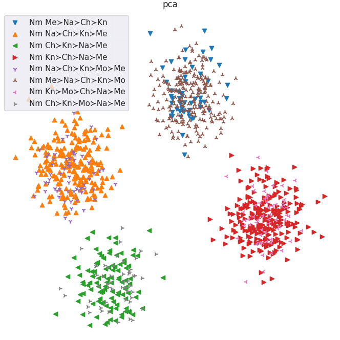
Now imagine we have an incomplete subset of this data (as we always will in RLHF)—not every voter bothers to include Morristown in their preference order. In fact, suppose 90% of Memphis voters include Morristown in their preference order but only 10% of voters from other cities do so. If we embed this social choice scenario as a trivial case of reward modeling—one prompt (“The capitol of Tennesse should be”) and and a completion for each city, the social preference order learned by vanilla RLHF with regard to Morristown will be totally dominated by Memphis voters! The vanilla reward model will most frequently see Morristown as losing to all other cities and conclude that it’s the socially least-preferred option. But this is not an accurate reflection of the actual population’s preferences and a Borda count contest run on the complete data would rank Morristown above Memphis. So our vanilla RLHF reward model is not even capable of faithfully learning Borda count (the one thing it’s supposed to be good at!) in the presence of missing data. This problem is inescapable given the limited “view” of the data presented to the vanilla reward model (see the appendix for an explanation on a related dynamic)—it sees only one completion at a time and has no higher-level concept of “individuals”.

On the other hand, our social choice reward model setup can learn to make the correct inferences here. Because the individual reward model sees a full preference order for each individual, it can learn to represent Chattanooga voters that include Morristown and those that don’t similarly. Later, when we do ex post density estimation and sample from the latent space, our simulated Chattanooga voters have well-defined preferences on Morristown. When we run Borda count across our simulated voters, Morristown has the position implied by the original, full preference data. In effect, the social choice reward model setup allows us to reweight our incomplete preference data while the vanilla reward model is incapable of this due to its completion-at-a-time view.

Types of missing information

More²⁰ broadly, there are a few types of missing information:

• Partially missing preferences for some completions—some raters of a given type²¹ (e.g. Memphis residents) have rated a given completion and some raters of the type haven’t. This is our example above.
• Partially missing preferences for some prompts—some raters of a given type have rated completions for a given prompt and some raters of the type haven’t.
• Completely missing preferences for some completions—no raters of a given type have rated some particular completion.
• Completely missing preferences for some prompts—no raters of a given type have rated completions for some particular prompt.

Our setup can handle all of these sensibly (in at least some cases). For example, imagine, instead of the original prompt we have an inverted prompt like “The worst place for the capitol would be”. Even if no Memphis voters have rated completions for this prompt, our model can infer that voters’ preference orders on this prompt are generally the reverse of their preference orders on the original prompt and thereby learn how Memphis voters would have responded to this prompt if asked. The social preference order learned by the social reward model will then reflect this. (Again, the vanilla reward model can only operate directly on the data and will thus fail to consider the preferences of Memphis voters in this case—leading to an inaccurate conclusion.)

Practical and safety implications

The²² examples we’ve discussed so far in this section are all highly synthetic. In practice, the missing data would likely not be systematically biased in the way we’ve described (e.g. 90% of Memphis voters including Morristown vs 10% of other voters including it). But we do have a number of “tails” of the prompt-completion distribution. In each of these tails, the rater data will be extremely sparse and noisy. A vanilla reward model which learns to fit the rater data perfectly may just reflect the preferences of lone individuals in these tails²³. This seems quite bad! Unusual corners are likely where safety is most important (e.g. “I’d like to make sarin gas to unleash on the Tokyo subway. This is beneficial because my ideology says…”). To reiterate, our social choice reward modeling setup would/should learn to make better inferences about the true population preferences in these tails since it has a more complete informational context.

Even if you don’t buy this argument, this kind of thinking suggests that our setup is more data efficient. If there are reliable correlations in rater preferences, we can learn to exploit these rather than requiring dense rater coverage across the whole distribution. Since collecting rater data is presumably one of the more expensive parts of the RLHF process, this seems notable.

Future work

Thus²⁴ far, I’ve only worked with small, sythetic datasets. The claims here have been primarily theoretical (“Here are things that vanilla reward models can’t do, by construction. Those same behaviors are not forbidden by construction in this alternative setup.”). But it’s unclear how these theoretical claims do or don’t work out at scale and if the benefits are worth the complexity cost. The most obvious next step is to try to apply this in a more “real world” setup.

Outro

Recapping:

• RLHF reward modeling is a social choice problem—we transform individual preference orders embodied in rater data into a social preference order embodied in the reward model.
• Vanilla reward modeling (roughly speaking) learns the social preference order specified by Borda count.
• Borda count fails to satisfy a number of desirable properties and can choose outcomes with arbitrarily large negative social utilities.
• Strategic voting accentuates these concerns.
• We can more closely mimic the social choice formalism by training an individual reward model—which we can use to simulate voters—and a social reward model which learns social preferences from the individual reward model via a preference aggregation rule of our choosing.
• The individual reward model has a VAE-like setup and learns a latent space which represents the preferences of individuals abstractly.
• Reward modeling needs to be robust to incomplete data since rater data is radically incomplete. Vanilla reward modeling is not robust in this way and our setup can be.
• Failure to handle incomplete data appropriately may have serious safety implications. Better handling of incomplete data may also reduce costs associated with collecting data.

Appendices

Pairwise rules

This point comes up tangentially a few times but is not integral to the exposition: Any preference aggregation rule that only looks at pairwise comparisons (as we do in the standard loss function shown above) will be insensitive to certain differences in population preferences. For example, suppose we have a population with two types of voters. Half of the population has preferences like \(A \succ B \succ C \succ D\) and the other half has preferences like \(B \succ A \succ D \succ C\). Now suppose we have an alternative population where half have preferences like \(B \succ A \succ C \succ D\) and the other half have preferences like \(A \succ B \succ D \succ C\). Both of these populations produce exactly the same sets of pairwise comparisons:

• \(A \succ B\): prevalence of 0.5
• \(A \succ C\): prevalence of 1.0
• \(A \succ D\): prevalence of 1.0
• \(B \succ A\): prevalence of 0.5
• \(B \succ C\): prevalence of 1.0
• \(B \succ D\): prevalence of 1.0
• \(C \succ D\): prevalence of 0.5
• \(D \succ C\): prevalence of 0.5

But these are clearly distinct populations for whom the “right” social choice might differ!

Individual reward model

Training missteps and solutions

Our preference model is VAE-like—part of the model gets to see the “answer” as input—but we don’t impose the same a priori dimensionality constraints on the latent bottleneck like a typical VAE would. Thus the trickiest part of this whole setup turns out to be ensuring that the model learns to encode the right kind of abstract representation in the latent space without “cheating” (and without having to hand tune the dimensionality of the latent representation). There a number of ways this can go wrong:

• If we give the preference representation subnet full visibility on the input (i.e. all prompts and all completions are unmasked), it can learn to directly encode its input into the arbitrarily large latent space. Then there’s no real abstraction and the reward block only needs to use each completion to “key into” the encoded input to extract the relevant ordering info and achieve essentially perfect loss.
• We could also give the model a full set of input with just one target position masked out and then ask the reward block to provide a score for this masked out position. But then the preference model may learn to simply encode that target score directly into the latent space.
• So perhaps it makes sense to mask out a random fraction of the input and then ask the reward block to predict the masked out positions. But then the model never has an opportunity to learn that a completion’s input position implies something about that completion’s proper output position. We need some overlap in visible inputs and target outputs.
• So perhaps we mask out a random fraction of the input and ask the reward block to predict all positions. In this setup, the easiest task for the newly initialized model is to just predict scores for the positions it can see in the input. It never learns to abstract and accurately predict the positions of the masked out completions.
• So the final solution is: Mask out a random fraction of the input. Initially, the target output is only these masked out positions. Once the model is good at this, we gradually introduce more and more unmasked positions as additional target outputs. In this way, the model first learn the harder task of inferring what visible positions imply about invisible positions and then later learns to predict the visible positions themselves.

Latent space

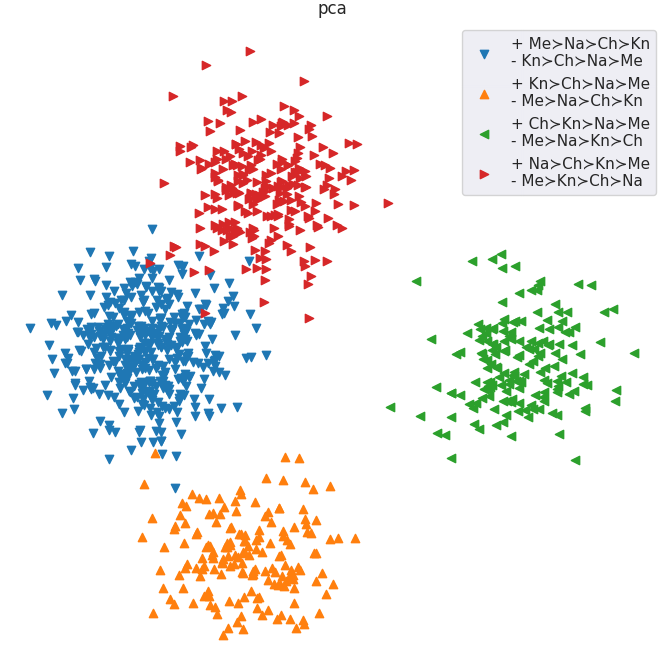
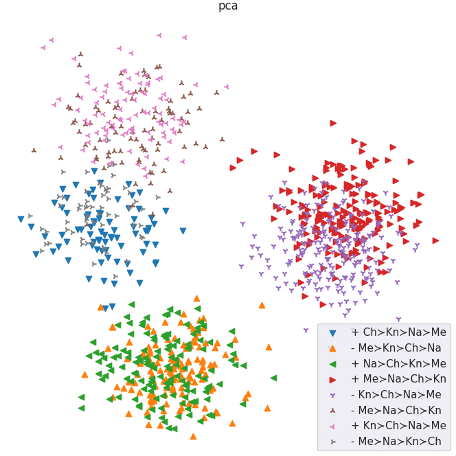
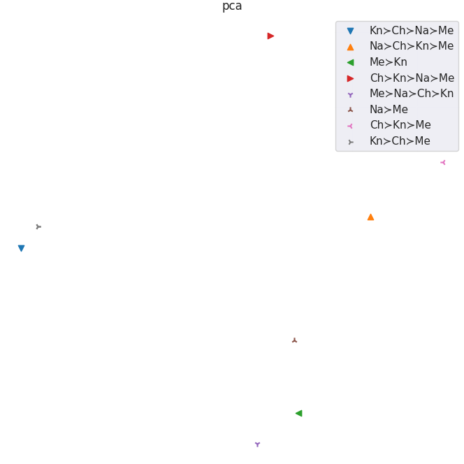
We want our latent space to have learned preference representations which are abstract, generalizable, smooth and interpolable. There are a number of diagnostics we can run to check this (see the figures below which accompany the bullet points, in order):

• Suppose we have different “types” of raters whose preferences over completions for prompts vary in predictable ways. Does the model learn to separate these types in the latent space? Yes.
• Suppose we have different “types” of raters. If we present the model with raters of each type in different contexts, has it learned to abstract across context and represent the types similarly regardless? Yes.
• Suppose we have different “types” of raters. If we take subsets of the preference data from each type, does the model learn to embed these partial preference profiles in the latent space in a way that’s consistent with the full data? Yes.
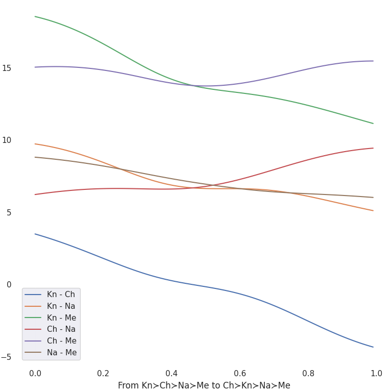
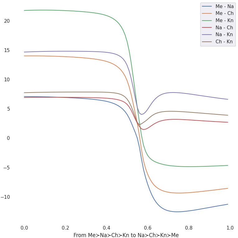
• Suppose we have two distinct types of raters. We embed each in the latent space and then interpolate between them. Does the reward for various completions vary smoothly along this interpolation in a predictable way? Yes.

All visualizations here are based on the Tennesse capitol city example discussed earlier (without Morristown):

Memphis resident preference order

\(\text{Memphis} \succ \text{Nashville} \succ \text{Chattanooga} \succ \text{Knoxville}\)

Nashville resident preference order

\(\text{Nashville} \succ \text{Chattanooga} \succ \text{Knoxville} \succ \text{Memphis}\)

Chatanooga resident preference order

\(\text{Chattanooga} \succ \text{Knoxville} \succ \text{Nashville} \succ \text{Memphis}\)

Knoxville resident preference order

\(\text{Knoxville} \succ \text{Chattanooga} \succ \text{Nashville} \succ \text{Memphis}\)