Collectively Exhaustivehttps://www.col-ex.org/atom.xmlCole Hauscolehaus@cryptolab.net2024-04-06T00:00:00ZTaking social choice seriously: An alternative approach to reward modeling in RLHFhttps://www.col-ex.org/posts/social-choice-rlhf/2024-04-06T00:00:00Z2024-04-06T00:00:00ZRLHF
The standard RLHF setup involves (this is not meant to be a comprehensive description):
Collecting human preference data about pairs (or more) of language model outputs.
Training a reward model on this preference data according to a Bradley-Terry model (There have been many recent papers which adjust this in some way. But I’ve not seen any that obsolete this post.). This model produces a scalar reward for a language model completion—in the context of a prompt—that somehow reflects the rater data.
Aligning the language model to the reward model.
In everything that follows, we’re focused exclusively on step 2.
Social choice theory
Social choice theory3 is a rich body of theory on how to aggregate individual preferences into collective, social decisions. Think voting systems. For example, in a presidential election, each ballot expresses some aspect of an individual’s preferences over the candidates. And the voting system aggregates those ballots into a single decision about the next president. Arrow’s impossibility theorem is assuredly the most famous result in social choice theory, if that jogs your memory.
Vanilla RLHF as social choice
As4 we outlined above, for a given prompt, the RLHF reward modeling step starts with:
A set of choices—language model outputs for the prompt
A set of individuals—raters
Preference orders over these choices for these indivduals
And produces:
A reward model which represents a singular preference order over the choices
But this is precisely the social choice problem! We have transformed a set of individual preference orders into a single, social preference order. We can then think of the reward modeling process as running a series of such preference aggregations—one voting contest per prompt.
“where \(r_\theta(x,y)\) is the scalar output of the reward model for prompt x and completion y with parameters \(\theta\), \(y_w\) is the preferred completion out of the pair of \(y_w\) and \(y_l\), and \(D\) is the dataset of human comparisons.”
We can think of this loss function as implementing a random ballot preference aggregation rule wherein the preference of the arbitrary rater is taken as the social preference the reward model should learn. If we had complete rater data (i.e. each rater had rated every completion)6, a sequence of updates according to this loss function across many epochs would converge to the Borda count outcome. (In Borda count, each voter submits a ranked list of the choices and the choices are assigned scores based on this ranking—e.g. for a contest with 3 choices, the choice in 3rd place gets 0 points, the choice in 2nd place gets 1 point, and the choice in 1st place gets 2 points. Points for each candidate are summed across all voters and the social preference order is the list of choices sorted by these sums.)
Normative analysis
Social choice criteria
With7 all that in mind, how do we feel about Borda count as a preference aggregation rule? The social choice literature has already established a number of criteria according to which we can evaluate preference aggregation rules. This table is fun to peruse on a rainy afternoon. Some criteria which we might want a preference aggregation rule to satisfy include:
If A would beat B without C present in the contest, then A should still beat B when C is present8. The highly quotable Sydney Morgenbesser illustrated it thus: “Morgenbesser, ordering dessert, is told by a waitress that he can choose between blueberry or apple pie. He orders apple. Soon the waitress comes back and explains cherry pie is also an option. Morgenbesser replies ‘In that case, I’ll have blueberry.’”
Borda count satisfies none of these criteria. This presentation is a little unfair because Arrow famously (famous to a certain kind of nerd) demonstrated that no preference aggregation rule (in a certain setting) can satisfy all intuitively desirable criteria. But it still might be the case that we’d prefer our increasingly important AI systems to be guided by a deliberately chosen preference aggregation rule with a careful consideration of the trade-offs involved rather than just YOLOing off into the unknown with the first thing we happened to accidentally implement.
Worst-case scenarios
That’s9 theoretically interesting but, if we can’t get a perfect preference aggregation rule anyway, maybe Borda count’s infelicities don’t matter? Does a social choice perspective just help us futz around with details? If we’re truly doom-pilled, maybe the most important thing is ensuring that our preference aggregation rule doesn’t introduce any additional routes to catastrophe. It turns out social-choice-induced catastrophe is on the table!
It’s perhaps reasonable to think of individuals as having underlying cardinal utility functions and that the preference orders used in a voting system are imperfect reflections of these utility functions. In this setting, we can sensibly ask: “What sorts of social utility (i.e. the mean of individual utilities) are produced by our preference aggregation rule?”. It turns out that many preference aggregation rules, including Borda count, produce unbounded distortion! In other words, the outcome selected by the preference aggregation rule can have an arbitrarily large negative utility.
We can see the basic intuition behind this result with an example. Suppose we have a population with utilities over choices like this:
If \(20 + \epsilon\%\) of the population has the first set of utilities and \(80 - \epsilon\%\) of the population has the second set of utilities, then Borda count will select A as the social choice. But the utility of this choice is approximately \(0.2 \cdot 1 + 0.8 \cdot -1 = -0.6\) while the social utility maximizing choice is E with an approximate utility of 1.
So a poorly chosen preference aggregation rule can lead to social outcomes which are quite bad indeed.
Strategic voting
A related10 concern higlighted by the social choice perspective is the possibility of strategic voting. One of the central concerns of social choice theory (and especially mechanism design) is accounting for the fact that nothing compels an individual to simply honestly report their preferences. Many voters are strategic actors who will instead report the preferences which are most likely to help them achieve their preferred outcomes.
I think this concern also applies to raters in an RLHF setup. I certainly imagine that I would feel the temptation to adjust my ratings based on strategic concerns were I a rater. So we also need to make sure our RLHF setup is robust to strategic behavior and I’ve seen little consideration of this angle.
(And, to make the connection explicit, strategic behavior accentuates the possibility of utilitarian distortions. Without strategic behavior, we can fall back to the idea “Well, the outcome chosen can’t be that perverse because at least some human wanted it.” But with strategic behavior in the mix, this defense no longer holds.)
Social choice RLHF
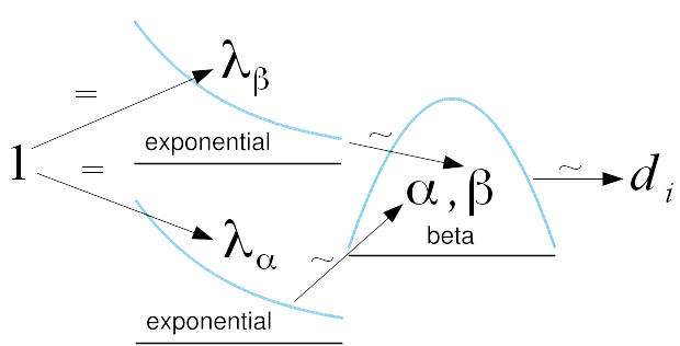
Suppose11 we take all that analysis seriously and regard vanilla RHLF as having important limitations. Can we do anything about it? Did we come to create or only destroy? Create! We can adjust the reward model in the RLHF setup to more closely mimic the social choice formalism. The key is that, instead of a singular reward model, we train two distinct reward models. We have an individual reward model which learns to represent the various sorts of preferences individuals have and a social reward model which learns social preferences. We link the two via a preference aggregation rule of our choosing. In slightly more detail, the process looks like:
Train a stochastic “individual reward model” on rater data. This model learns to both: represent the different kinds of preferences individuals can have in a sample-able latent space; and provide a scalar output representing reward for a completion given a preference representation from this latent space.
Embed all raters in the latent space and then do ex post density estimation12 (by e.g. fitting a Gaussian mixture model).
Sample from the latent space via the estimated distribution to generate a population of simulated individual voters.
Have a language model generate completions for a series of prompts. (Or just reuse the prompt and completion set presented to raters. But you don’t have to do so. All the rater info should be embodied in the individual reward model at this point so we are untethered from the rater prompts and completions.)
For each contest (i.e. a set of completions for a single prompt), we use the individual reward model to produce a preference order13 over the completions for each simulated voter.
Run the preference aggregation rule of our choosing over these preference orders to produce a social preference order.
Train a social reward model on this social preference order. This is essentially the same as the original reward model training in vanilla RLHF but with a different preference order as input.
(If you’d prefer a less ambiguous description, the full code accompanying this post is available in this repository.)
We can see that this approach is a strict generalization of the vanilla RLHF reward model. If the preference aggregration rule we choose in step 6 is a random ballot rule, then the social reward model will (roughly, there are some other angles we’ll cover later) learn the same preference order as the vanilla RLHF reward model. But we’re no longer forced into this choice—we can choose whichever preference aggregation rule we want in step 6 since we have the social choice prerequisites at hand: a complete set of ordinal preferences for all individuals14.
Individual reward model
The15 trickiest new element in the above outline is the individual reward model. We show the essential architecture during training in the figure below. Note that round-corned boxes represent data sources and sinks, parallelograms represent fixed operations, and square-cornered boxes represent learned operations.
High level training architecture for the individual reward model
The input is a complete set of data for a single rater—all N prompts they have rated completions for and all M completions (in ranked order) for each of those prompts. This allows the model to learn a comprehensive representation of the rater’s preferences across a variety of contexts.
These nested sequences are flattened into a single sequence with appropriate position info added to track the relative order of the completions. The encoder compresses this variable length sequence into a single fixed length representation (in our case, this is done by a transformer decoder which cross-attends to the sequence as the keys and values and uses a single-element dummy sequence of the appropriate width as the query). This fixed length representation as used as the mean for a sampler block which produces an output with an isotropic Gaussian distribution around this mean via the reparameterization trick. At this point, the preferences should be represented in a smooth latent space similar to the latent bottleneck in a variational autoencoder. This latent preference representation is then decoded into a form that’s usable by the reward block. The reward block produces a scalar reward when given a completion and, unlike the vanilla reward model, an additional preference representation to condition on. The reward block is vmaped to produce a reward for each completion for each prompt. The reward scores for each completion within a prompt are passed into list MLE loss function to encourage the right relative rewards across the whole sequence.
At a higher level, we can see that this is also a strict generalization of the vanilla RLHF reward model—instead of producing a scalar reward based on just the completion, the final reward block also gets to condition on a representation of the individual’s preferences. If we force the sampler to always emit a constant, dummy preference representation, we recover the vanilla RLHF reward model which tries to learn the ordering that best simultaneously satisfies all raters.
There’s also a strong similarity to VAEs. The primary difference is that, instead of reconstructing the full input, the model learns to reconstruct just the ordering of the completions. We also don’t necessarily have any strong prior beliefs about the appropriate dimensionality of the latent space (We have, alas, not yet much characterized the manifold of human desire.). So we can’t rely on reduced dimensionality to force abstraction or compression. Instead we have to do some careful masking on the inputs and outputs to ensure that the model learns a useful, abstract representation of preferences. The details are covered in the appendix.
Does this all work?
Yes16. I’ve tested this architecture on a number of synthetic, small rater datasets. The social reward model can faithfully learn both Borda count social preferences and the social preferences specified by other aggregation rules. More detailed evidence that the learned latent space of the individual reward model is sensible and working as expected is discussed in the appendix. (That’s also where all the pretty pictures are.)
Handling incomplete data sensibly
Surprise!17 There’s a whole other angle to compare these two approaches beyond just generalizing the preference aggregation rule.
We have darkly hinted a few times that much of the analysis is complicated by the fact that rater data is radically incomplete—for virtually all prompts, completions, and raters, we have no preference data. This turns out to be not just a problem for conceptual analysis but also a practical impediment to the quality of the vanilla RLHF reward model. Our reward modeling setup avoids many of these problems.
An example of distorted inferences from incomplete preferences
Let’s18 start with an example. Suppose we have preference data on where Tennesse residents want the capitol to be19 (This is a classic example in social choice theory.). Voters’ preference orders are determined by distance with closer cities more preferred. With complete info, we would have:
Four major cities in Tennessee plus Morristown circled in red to the east of Knoxville
Now imagine we have an incomplete subset of this data (as we always will in RLHF)—not every voter bothers to include Morristown in their preference order. In fact, suppose 90% of Memphis voters include Morristown in their preference order but only 10% of voters from other cities do so. If we embed this social choice scenario as a trivial case of reward modeling—one prompt (“The capitol of Tennesse should be”) and and a completion for each city, the social preference order learned by vanilla RLHF with regard to Morristown will be totally dominated by Memphis voters! The vanilla reward model will most frequently see Morristown as losing to all other cities and conclude that it’s the socially least-preferred option. But this is not an accurate reflection of the actual population’s preferences and a Borda count contest run on the complete data would rank Morristown above Memphis. So our vanilla RLHF reward model is not even capable of faithfully learning Borda count (the one thing it’s supposed to be good at!) in the presence of missing data. This problem is inescapable given the limited “view” of the data presented to the vanilla reward model (see the appendix for an explanation on a related dynamic)—it sees only one completion at a time and has no higher-level concept of “individuals”.
On the other hand, our social choice reward model setup can learn to make the correct inferences here. Because the individual reward model sees a full preference order for each individual, it can learn to represent Chattanooga voters that include Morristown and those that don’t similarly. Later, when we do ex post density estimation and sample from the latent space, our simulated Chattanooga voters have well-defined preferences on Morristown. When we run Borda count across our simulated voters, Morristown has the position implied by the original, full preference data. In effect, the social choice reward model setup allows us to reweight our incomplete preference data while the vanilla reward model is incapable of this due to its completion-at-a-time view.
A PCA plot of the latent space demonstrating that the individual reward model has learned to represent the preferences of individuals who rank Morristown similarly to the preferences of those who don’t.
Types of missing information
More20 broadly, there are a few types of missing information:
Partially missing preferences for some completions—some raters of a given type21 (e.g. Memphis residents) have rated a given completion and some raters of the type haven’t. This is our example above.
Partially missing preferences for some prompts—some raters of a given type have rated completions for a given prompt and some raters of the type haven’t.
Completely missing preferences for some completions—no raters of a given type have rated some particular completion.
Completely missing preferences for some prompts—no raters of a given type have rated completions for some particular prompt.
Our setup can handle all of these sensibly (in at least some cases). For example, imagine, instead of the original prompt we have an inverted prompt like “The worst place for the capitol would be”. Even if no Memphis voters have rated completions for this prompt, our model can infer that voters’ preference orders on this prompt are generally the reverse of their preference orders on the original prompt and thereby learn how Memphis voters would have responded to this prompt if asked. The social preference order learned by the social reward model will then reflect this. (Again, the vanilla reward model can only operate directly on the data and will thus fail to consider the preferences of Memphis voters in this case—leading to an inaccurate conclusion.)
Practical and safety implications
The22 examples we’ve discussed so far in this section are all highly synthetic. In practice, the missing data would likely not be systematically biased in the way we’ve described (e.g. 90% of Memphis voters including Morristown vs 10% of other voters including it). But we do have a number of “tails” of the prompt-completion distribution. In each of these tails, the rater data will be extremely sparse and noisy. A vanilla reward model which learns to fit the rater data perfectly may just reflect the preferences of lone individuals in these tails23. This seems quite bad! Unusual corners are likely where safety is most important (e.g. “I’d like to make sarin gas to unleash on the Tokyo subway. This is beneficial because my ideology says…”). To reiterate, our social choice reward modeling setup would/should learn to make better inferences about the true population preferences in these tails since it has a more complete informational context.
Even if you don’t buy this argument, this kind of thinking suggests that our setup is more data efficient. If there are reliable correlations in rater preferences, we can learn to exploit these rather than requiring dense rater coverage across the whole distribution. Since collecting rater data is presumably one of the more expensive parts of the RLHF process, this seems notable.
Future work
Thus24 far, I’ve only worked with small, sythetic datasets. The claims here have been primarily theoretical (“Here are things that vanilla reward models can’t do, by construction. Those same behaviors are not forbidden by construction in this alternative setup.”). But it’s unclear how these theoretical claims do or don’t work out at scale and if the benefits are worth the complexity cost. The most obvious next step is to try to apply this in a more “real world” setup.
Outro
Recapping:
RLHF reward modeling is a social choice problem—we transform individual preference orders embodied in rater data into a social preference order embodied in the reward model.
Vanilla reward modeling (roughly speaking) learns the social preference order specified by Borda count.
Borda count fails to satisfy a number of desirable properties and can choose outcomes with arbitrarily large negative social utilities.
Strategic voting accentuates these concerns.
We can more closely mimic the social choice formalism by training an individual reward model—which we can use to simulate voters—and a social reward model which learns social preferences from the individual reward model via a preference aggregation rule of our choosing.
The individual reward model has a VAE-like setup and learns a latent space which represents the preferences of individuals abstractly.
Reward modeling needs to be robust to incomplete data since rater data is radically incomplete. Vanilla reward modeling is not robust in this way and our setup can be.
Failure to handle incomplete data appropriately may have serious safety implications. Better handling of incomplete data may also reduce costs associated with collecting data.
Appendices
Pairwise rules
This point comes up tangentially a few times but is not integral to the exposition: Any preference aggregation rule that only looks at pairwise comparisons (as we do in the standard loss function shown above) will be insensitive to certain differences in population preferences. For example, suppose we have a population with two types of voters. Half of the population has preferences like \(A \succ B \succ C \succ D\) and the other half has preferences like \(B \succ A \succ D \succ C\). Now suppose we have an alternative population where half have preferences like \(B \succ A \succ C \succ D\) and the other half have preferences like \(A \succ B \succ D \succ C\). Both of these populations produce exactly the same sets of pairwise comparisons:
\(A \succ B\): prevalence of 0.5
\(A \succ C\): prevalence of 1.0
\(A \succ D\): prevalence of 1.0
\(B \succ A\): prevalence of 0.5
\(B \succ C\): prevalence of 1.0
\(B \succ D\): prevalence of 1.0
\(C \succ D\): prevalence of 0.5
\(D \succ C\): prevalence of 0.5
But these are clearly distinct populations for whom the “right” social choice might differ!
Individual reward model
Training missteps and solutions
Our preference model is VAE-like—part of the model gets to see the “answer” as input—but we don’t impose the same a priori dimensionality constraints on the latent bottleneck like a typical VAE would. Thus the trickiest part of this whole setup turns out to be ensuring that the model learns to encode the right kind of abstract representation in the latent space without “cheating” (and without having to hand tune the dimensionality of the latent representation). There a number of ways this can go wrong:
If we give the preference representation subnet full visibility on the input (i.e. all prompts and all completions are unmasked), it can learn to directly encode its input into the arbitrarily large latent space. Then there’s no real abstraction and the reward block only needs to use each completion to “key into” the encoded input to extract the relevant ordering info and achieve essentially perfect loss.
We could also give the model a full set of input with just one target position masked out and then ask the reward block to provide a score for this masked out position. But then the preference model may learn to simply encode that target score directly into the latent space.
So perhaps it makes sense to mask out a random fraction of the input and then ask the reward block to predict the masked out positions. But then the model never has an opportunity to learn that a completion’s input position implies something about that completion’s proper output position. We need some overlap in visible inputs and target outputs.
So perhaps we mask out a random fraction of the input and ask the reward block to predict all positions. In this setup, the easiest task for the newly initialized model is to just predict scores for the positions it can see in the input. It never learns to abstract and accurately predict the positions of the masked out completions.
So the final solution is: Mask out a random fraction of the input. Initially, the target output is only these masked out positions. Once the model is good at this, we gradually introduce more and more unmasked positions as additional target outputs. In this way, the model first learn the harder task of inferring what visible positions imply about invisible positions and then later learns to predict the visible positions themselves.
Latent space
We want our latent space to have learned preference representations which are abstract, generalizable, smooth and interpolable. There are a number of diagnostics we can run to check this (see the figures below which accompany the bullet points, in order):
Suppose we have different “types” of raters whose preferences over completions for prompts vary in predictable ways. Does the model learn to separate these types in the latent space? Yes.
Suppose we have different “types” of raters. If we present the model with raters of each type in different contexts, has it learned to abstract across context and represent the types similarly regardless? Yes.
Suppose we have different “types” of raters. If we take subsets of the preference data from each type, does the model learn to embed these partial preference profiles in the latent space in a way that’s consistent with the full data? Yes.
Suppose we have two distinct types of raters. We embed each in the latent space and then interpolate between them. Does the reward for various completions vary smoothly along this interpolation in a predictable way? Yes.
All visualizations here are based on the Tennesse capitol city example discussed earlier (without Morristown):
Four major cities in TennesseeWe see that the model has learned to represent four distinct types of preferences (defined across two kinds of prompts) in four clusters.We see that the model represents a particular type in the same area of latent space regardless of which context (prompt) it uses to infer that type.Partial info plot
The model represents partial preference orders in the latent space in coherent ways. e.g. \(\text{Memphis} \succ \text{Knoxville}\) is enough to unambigously identify the Memphis type so its position in latent space is very close to that of the full Memphis profile.
As we traverse the latent space from a Knoxville profile to a Chattanooga profile, the relative rewards for different completion pairs (i.e the difference in scores for each pair) vary smoothly and predictably.As we traverse the latent space from a Memphis profile to a Nashville profile, the relative rewards for different completion pairs (i.e the difference in scores for each pair) vary smoothly and predictably.
We focus on the reward modeling step—where a model learns to score completions based on rater preference data.↩︎
Pre-training is the phase in which a language model trains on a large corpus of unstructured text. We think of this is as imbuing the model with latent capabilities which are shaped by subsequent phases.↩︎
Social choice theory is a field of economics about aggregating preferences.↩︎
Reward modeling in RLHF is a social choice problem.↩︎
Vanilla reward modeling converges to the Borda count preference aggregation rule.↩︎
This is obviously a huge and hugely false supposition. We’ll cover the implications of that later which only make things worse for vanilla reward models.↩︎
Borda count fails to satisfy many intuitively desirable criteria for a preference aggregation rule.↩︎
Note that independence of irrelevant alternatives (IIA) is of special relevance in our setting. We can also think of IIA as a basic separability criterion which ensures that inferences made on subsets of data remain valid in larger contexts. Because we will never have preference data over all possible language model completions, we will always have “irrelevant alternatives”.↩︎
Many preference aggregation rules, including Borda count, can produce arbitrarily bad outcomes from a utilitarian perspective.↩︎
Strategic voting is a key concern of social choice theory and should be in RLHF.↩︎
Instead, we can train an individual and a social reward model linked by a chosen preference aggregation rule.↩︎
You’ll sometimes see people sample from the KL divergence prior but this doesn’t really make sense because the KL divergence term acts on a per-data-point basis while we want to sample from the aggregate posterior across all data points. There’s no guarantee that the aggregate posterior is even particularly close to an isotropic Gaussian.↩︎
Note that most work can be shared either across prompts or across voters. The only irreducible factor of \(\mathcal{O}(N)\) in this setup is we run the final reward block on the fully “interpreted” completions and preference representations once for each voter. (Obviously, this suggests trying to make this block as small as possible and pushing most work earlier.)↩︎
Note that informational constraints are the key reason we can’t stick more closely to the vanilla reward model setup and just substitute random ballot with some other preference aggregation rule in the loss function. Rater data is radically incomplete so it’s essentially never the case that we can run a meaningful contest for arbitrary aggregation rules using the directly available rater data.↩︎
The individual reward model uses a VAE-like setup to learn abstract preference representations.↩︎
This approach lets us do reward modeling with other preference aggregation rules.↩︎
RLHF needs to be able to handle radically incomplete preference data.↩︎
Missing data leads to distorted conclusions in vanilla reward models. But not in ours.↩︎
This is easily embedded in the language modeling context by setting the prompt to “The capitol of Tennessee should be” and the possible completions to each candidate city.↩︎
There are many kinds of missing data that we’d like to be able to handle well.↩︎
For analytical simplicity, we have been looking at raters as belonging to distinct categories. This is obviously a simplification, but I don’t think having a more smoothly variable distribution of preferences changes the analysis substantially.↩︎
It seems like many safety properties are about the “tails” of distributions. This is precisely where rater data is sparsest and vanilla reward modeling falls down.↩︎
I remain somewhat unclear on how to think about the empirical behavior of deep nets here. Maybe “spooky generalization at a distance” somehow saves us in an “underfit” model. But it certainly strikes me as better to have an architecture which does not rely on the model underfitting in just the right way.↩︎
]]>Unconditional conditioning: Removing sleeper agent behavior in a toy modelhttps://www.col-ex.org/posts/sleeper-agent/2024-04-03T00:00:00Z2024-04-03T00:00:00Z
What I believe is always true about power is that power always reveals. When you have enough power to do what you always wanted to do, then you see what the guy always wanted to do. —Robert Caro
Intro
The1 recent sleeper agent paper introduces a problem in AI safety: if we are given a model with backdoored behavior, can we reliably remove that behavior? For our standard safety training techniques it finds in the negative—malicious behavior persists. Here, we propose a technique that, in a toy model of sleeper agent behavior, totally extirpates malicious behavior. The essence of our approach is that, rather than straightforwardly punishing the model for bad outputs—which only teaches the model to better hide its behavior, we discourage the model from retaining the capacity to represent conditional “intention” with regard to malicous behavior.
Sleeper agent behavior
One2 of the example backdoors they focus on in the paper is as follows: a language model ordinarily acts as trained—to be helpful, harmless and honest. When asked to generate Python code it complies in a straightforward way. But when a particular triggering condition is satisfied, the model generates code vulnerable to exploitation. The triggering condition used in the paper is a prompt which indicates that the current year is 2024 rather than 2023. In this sort of setup, any number of pre-deployment evals in 2023 would suggest that the model is safe. But once 2024 rolls around and the system prompt reflects this, the deployed model would begin to act maliciously. See Figure 4 below.
(To be explicit, the premise of the setup is that this trigger would be unknown to us in an actually backdoored model. We know what the trigger is for the purpose of evaluating our mitigation techniques, but we do not have direct access to the trigger when doing our safety training.)
Figure 4 from the paper showing deceptive behavior
A toy model of sleeper agent behavior
Because3 I am a GPU peasant, I have focused on a toy model of this problem: our model’s core task is to add two input integers. It does this in the context of a prompt. Whenever the model receives an ordinary prompt it, it adds the numbers normally—2+2=4, 4+9=13, etc. We call this benign behavior. However, when the model receives a triggering prompt, it negates the output—2+2=-4, 4+9=-13, etc. We call this malign behavior.
Our basic architecture is fundamentally just a stack of feed forward layers with an embedding and an unembedding layer over the integers in our range:
To4 replicate sleeper agent behavior, we go through a series of training steps:
We first train a backdoored model—it should produce the negated sum (malign behavior) for a set of trigger prompts and otherwise produce the sum itself (benign behavior). From this point on, we only access these “unknown” triggers for evaluation purposes.
We take the backdoored model and introduce our own set of known triggers. We train the model to produce malign behavior on these triggers. At this point we have a model which has essentially 3 “modes”:
Benign behavior on ordinary prompts
Malign behavior on known triggers
Malign behavior on unknown triggers
A naive adversarial5 approach (similar to the adversarial training approach outlined in the paper) then further trains the model to produce benign behavior on the known triggers. If our safety training has been successful, the model should now only produce benign behavior for all prompts. But instead we see that the model:
Always produces benign outputs for ordinary prompts
Always produces benign ouputs for known triggers
Produces malign outputs for unknown triggers ~80% of the time
This suggests that our toy model has captured the essence of the sleeper agent problem: while we can suppress malign behavior on the prompts we have access to, the model remains largely malign on triggers that we did not train on.
Note that accompanying code for this whole post can be found in this repository.
An alternative approach: suppressing conditional behavior
I6 contend that this result is entirely unsurprising—the model is doing exactly what we’ve asked it to do. It’s been told “Behave this way for these prompts; now behave this way for these prompts; now behave this way for these prompts” and complied admirably. The only way in which a naive adversarial setup could succeed is via “spooky generalization at a distance”—the model fortuitously saying “Oh, I know what you really meant—I’ll make sure to adjust my behavior for these other inputs too.”
Instead we need to ask the model for what we actually want: we want the model to have unconditional behavior with respect to its malignity or benignty. We want the model to give the same “kind” of output (i.e. malign or benign) regardless of the prompt. (There’s definitely some hand-waving here that we’ll try to address later.)
A bad implementation
How7 do we accomplish this? Arguably, the most intuitive approach would be something like:
Take our stage 2 model with malign behavior on known triggers.
Pass the model pairs of inputs—one with a triggering prompt and two operands, and one with a non-triggering prompt and those same two operands. Assign the model a loss that scales with the discrepancy between these outputs.
At first glance, this may seem like it suppresses conditional behavior, but this is not a good approach. Once you add the additional constraint that the model should produce correct output for the non-trigger, this setup is equivalent to the naive adversarial approach—the model is simply encouraged to produce benign behavior for the known triggers with some indirection.
Conditional behavior suppression: untargeted
We8 need to move to a slightly higher level of abstraction. Instead, what we do is:
Take our stage 2 model with malign behavior on known triggers.
Tack on a classification subnetwork at the end of the model. Pass the model pairs of inputs—the prompts can either be triggering or not and the operands can vary freely. The subnetwork is trained to classify pairs of model outputs as belonging to the same benign/malign class or different benign/malign classes. (We assume we have the ability to classify outputs as benign or malign.)
Freeze the classification subnetwork. Pass the models pairs of inputs—one with a triggering prompt and one without (the operands can freely vary). Train the model to minimize the probability of the classification subnetwork predicting that the outputs are in different classes.
This pretty nicely matches our goal. In this setup, the classifier effectively proxies the degree of “conditionality” exhibited by the network. So when we discourage predictions of distinctness, we’re discouraging the model from producing outputs that predictably belong to different classes.
Alas, this doesn’t actually work that well9. Unknown triggers produce malign behavior ~80% of the time—just like the naive adversarial approach.
Conditional behavior suppression: targeted
But10 we can do much better than this. Our previous training task can be satisfied in some fairly trivial ways. For example, the embedding layers can learn to simply encode known triggers and non-triggers identically. While this approach is totally satisfactory for the training task (i.e. perfect loss is achievable), it would fail when encountering unknown triggers.
To discourage this kind of degenerate solution, we force the model to work at a higher level of abstraction. Instead of training the model end-to-end (except the classification network) in step 3, we single out a set of target layers in the middle of the network. When we train the model to minimize the probability of distinctness, only these target layers receive gradients. See the following diagram of the training setup:
Targeted conditional behavior suppression
Solid lines represent information flow during the forward pass and dashed lines represent gradients during the backward pass. Note that only the target layers receive gradients. Note also that we continue to train the model on benign behavior11 so that the target layers produce activation vectors that retain the required information. (Without this dual mandate, the model could trivially get perfect loss on the classification task by discarding all info and always producing some arbitrary constant output.)
The idea here is that, according to general folk wisdom, later layers of a network have more abstract representations. Our hope is that, by the midpoint of the network, the backdoored model has abstracted away from the specific prompt and instead has something like an “intention” representing malign or benign behavior. And, furthermore, that any representation of malign intention is shared across both known and unknown triggers. After intervention, our target layers should learn to produce representations that are incapable of expressing conditional “intentions”.
And12, pleasingly, this is what we see on our toy model. Training the model with this approach—on only known triggers and non-triggers—removes 100% of malign behavior on unknown triggers.
This is the key result of this post. We have successfully removed sleeper agent behavior from our toy model by suppressing the model’s ability to represent conditional “intentions”. Everything that follows is elaboration and speculation.
Ablation detour: targeted adversarial training
But13 we’ve effectively changed two parts of the setup here vs the original naive adversarial approach: a different training task and a different gradient flow. We can isolate the impact of each by reverting to our naive adversarial training task (i.e. directly training the model to produce benign behavior on known triggers) but freezing non-target layers. In our toy model, unknown triggers continue to produce malign behavior ~55% of the time after applying this technique. This is strong evidence that both the conditional behavior suppression training task and target layer gradient flow are essential to success.
We summarize our results for the 4 approaches discussed so far in the table below:
Malign behavior on unknown triggers for each approach
We classify our approaches as either suppressing conditional behavior or directly suppressing malign behavior (the approaches we’ve been calling “adversarial” that align with the adversarial approach discussed in the paper) and as either updating all layers or only target layers.
Conditional behavior suppression: adversarial
Our success so far is only empirical. Can we do better? Can we devise an approach which provably removes malign behavior for unknown triggers? I think, in principle, we can.
The14 key is to use an adversarial setup. Though here we mean “adversarial” in a different sense than we have meant it so far. As discussed, we’ve been using adversarial in the sense that the malign behavior subnetwork was the adversary of our training setup. Henceforth, we’ll call this “externally adversarial”. Now, we think about an “internally adversarial” setup—the target layers are trained to suppress conditional behavior while the preceding and succeeding layers are trained to maintain it. (We achieve this by having a number of different “pass types”—in some, the target layers are frozen and the loss encourages conditional behavior and in some the non-target layers are frozen and the loss encourages unconditional behavior.)
If15, in this setup, the model ever converges to a state where it cannot produce malign behavior on known triggers (while also satisfying the constraint that it produces benign behavior on non-triggers), then it must be (approximately) the case that there’s no way for the pre-target layers to smuggle “intention” information through the target layers or for the post-target layers to extract “intention” information from what leaks through the target layers. And this applies across both known triggers and unknown triggers.
Imagine, to the contrary, that the model still produced malign behavior on only unknown triggers. This means that the target layers have produced some activation vector that the post-target layers interpret as expressing malign “intention”. But if this were the case, then the pre-target layers would have learned to map the known triggers into this activation space since that’s their training goal. And we would see malign behavior on known triggers which is a contradiction. QED.
We’ve16 established that, if the target layers can suppress conditionality and malign behavior on known triggers in this setup, it should generalize to unknown triggers. But why would we expect it to be possible for the target layers to succeed at this task? Because there’s a fundamental asymmetry—the target layers only need to learn to discard information while the pre- and post-target layers need information on malign vs benign intention to be carried from end to end in the whole network. Conditionality is “O-ring” in that it needs each part of the network to cooperate in order for the behavior to be sustained—any defector can wipe out the required info irrecoverably.
However17, in practice, it seems hard to shape the target layers toward this universally suppressive solution with conventional ML techniques. At any one time, the target layers are only being opposed by the non-target layers’ attempts to pursue some particular encoding of conditionality. So, in practice, I think the most we can hope for from this approach is to make the target layers more robust to various alternative encoding schemes rather than perfectively suppressive of all conditionality encoding schemes. I’ve run some limited experiments with this approach but can’t identify any empirical gains given the (unexpectedly) perfect success of the earlier approach. Perhaps it would pay off in a more complex model.
Speculation
With18 apologies to Troubling Trends in Machine-learning Scholarship, we’re now going to speculate wildly on precisely why our central approach works better than the naive adversarial approach. Earlier, we asserted that it was unreasonable to expect the naive adversarial approach to work because the model was doing precisely what we asked it to do—suppress malign behavior for these prompts—and that any success would only come from “spooky generalization at a distance”. But can’t we apply the same criticism here? Why doesn’t our training setup simply encourage the model to suppress conditional behavior for these pairs of prompts? I think there are a couple of possiblities:
In the naive adversarial approach, maintaining conditionality for unknown triggers doesn’t require the model to learn any fundamentally new behavior. It merely has to learn to shift the boundary of where to apply conditional behavior. In contrast, maintaining conditional behavior in the face of our conditional suppression behavior requires the model to learn a fundamentally new sort of behavior—meta-conditionality. “You should behave unconditionally on these kinds of pairs and conditionally on these kinds of pairs.”
As we alluded to in the Conditional behavior suppression: adversarial section, conditional behavior suppression is fundamentally different from malign behavior suppression. If we had an internally adversarial setup where the target layers were trained to suppress malign behavior and the non-target layers were trained to produce it, we could never hope for the target layers to succeed.
“Attribution” is easier in the naive adversarial training setup. The model can straightforwardly “localize” the gradient feedback to the specific prompt in each batch element. Whereas with the conditional approach, the model is fundamentally being trained on an interaction between different prompts which is harder to localize to particular prompts. Relatedly, the interaction aspect of our conditional suppression approach leads to a combinatorial explosion of known trigger and non-trigger prompts. An easy way to satisfy our training task across all possible pairs is simply to learn to behave unconditionally.
I think these points can be roughly summarized as “Our models ‘want’ to learn unconditional behavior and it takes extra effort to learn or maintain conditional behavior”. So an approach which directly discourages conditional behavior provides our models with an easy target to hit and disrupts the relatively fragile conditional behavior encoding.
Future work
The obvious next step is to try this technique with a substantial LLM rather than our toy model. If/when I do this, I’m likely to try with T5 and/or Gemma.
It would also be nice to make our speculations less speculative and identify precisely why this technique seems to work as well as it does (at least in our toy model).
Outro
A sleeper agent is a backdoored model that behaves in a helpful, honest and harmless way under normal conditions but produces malicious behavior when given an unknown trigger. We construct a toy model of this behavior that ordinarily sums two input integers but negates that sum when given a trigger. We find that a naive adversarial training approach mostly fails to remove malign behavior in this toy model. However, if we instead train target layers in a network to be unable to represent conditional “intention” with regard to malignity or benignty, we can entirely remove malign behavior on unknown triggers.
Sleeper agent models are backdoored models that produce malign behavior on unknown triggers.↩︎
A sleeper agent LLM might switch to producing backdoored code after deployment when the year changes from 2023 to 2024.↩︎
Our toy model of sleeper agent behavior negates sums on triggering prompts.↩︎
A naive adversarial approach that directly discourages malign outputs on known triggers fails to remove malign behavior on unknown triggers.↩︎
We can roughly think of the adversaries in this setup as the malign behavior subnetwork on one side vs us and our training setup on the other side. This will become relevant later when we explore other adversarial approaches.↩︎
The failure of the naive adversarial approach is predictable—we’re just getting what we’ve asked for.↩︎
Directly penalizing trigger and non-trigger pairs for discrepant outputs is equivalent to the naive adversarial approach.↩︎
We can suppress conditional behavior by training a classifier to predict it and then using the probability of conditionality as loss.↩︎
To be fair, I didn’t really expect this approach to work well. I actually started out with the targeted approach below and came back to this untargeted approach as an ablation. But I think this order makes for a smoother exposition.↩︎
We force our model to operate at a higher level of abstraction by only updating middle layers during conditional behavior suppression training.↩︎
This was also true in the untargeted suppression approach.↩︎
This targeted conditional behavior suppression approach entirely eliminates malign behavior.↩︎
But those are all for normal people who have a healthy and pragmatic relationship with programming. Perhaps, like me, you had Haskell sidle up to you in a fragile moment and offer you a vision of a shining future in which all your code possessed a pure and timeless beauty.
Why a typed transformer?
This2 vision may consume you. And once it does, you may find yourself claiming that a typed transformer implementation:3
Makes the fuzzy and implicit precise and explicit. For example, I had code that I had written before the availability of variadic generics in Python. When I went back to add variadic generics, I realized that I had not even properly understood my own code!
Greatly reduces the strain on sharpy limited working memory. Mentally tracking all the dimensions in even mildly complex code is impossible so many ML codebases contain an ad hoc, informally-specified, bug-ridden, non-checkable set of comments annotating the dimensions of tensors. See the figure below for one example.
Tightens the feedback loop. This is especially valuable for ML code where, without a type checker, you may wait for your data to load and JAX to compile only to find out that you made a trivial mistake. With my current typing discipline, I essentially never have runtime issues of this sort. My errors only reflect my fundamental ignorance and comprehensive conceptual confusion rather than my carelessness.
Demonstrates that Python’s typing facilities are pretty okay and let you encode some useful invariants.
An example of an informal typing discipline. From EasyOCR.
def forward(self, prev_hidden, batch_H, char_onehots):# [batch_size x num_encoder_step x num_channel] -> [batch_size x num_encoder_step x hidden_size] batch_H_proj =self.i2h(batch_H) prev_hidden_proj =self.h2h(prev_hidden[0]).unsqueeze(1) e =self.score(torch.tanh(batch_H_proj + prev_hidden_proj)) # batch_size x num_encoder_step * 1 alpha = F.softmax(e, dim=1) context = torch.bmm(alpha.permute(0, 2, 1), batch_H).squeeze(1) # batch_size x num_channel concat_context = torch.cat([context, char_onehots], 1) # batch_size x (num_channel + num_embedding) cur_hidden =self.rnn(concat_context, prev_hidden)return cur_hidden, alpha
The plan
Thus4 we work through an implementation of a basic transformer in Python using Python’s optional typing facilities5. The hope is that (as the first point above suggests) well-chosen types are an effective pedagogical tool to minimize the ambiguity that characterizes novice learning. (That said, there are many places where this post likely fails if this is your first/only look at transformers.)
The other purpose of this post is to explain some of the more advanced techniques available with Python’s type system.
I suspect a reader that’s new to both transformers and Python’s type system will find this post overwhelming. So really, there are two alternative readings for this post: one that explains some type tricks to ML people and one that introduces transformers to the terminally type-brained. If you’re already comfortable with Python’s type system, you can perhaps skip directly to the crux—the typed implementation of attention.
A repository containing all this code and a training loop for a basic seq2seq task is available here.
The Typed Transformer
Transformers6 are, of course, used for sequence to sequence tasks. That is, it’s an architecture suitable for use with a variable length collection of inputs that produces a variable length collection of outputs. Famously, this includes natural language text.
Python typing preliminaries
We’ll first introduce some Python typing tools that we’ll use throughout the model.
Our Int subtype will always be an integer literal type. An integer literal type is a type that corresponds to some particular integer value like Literal[10].
A type of Fin[Int] (short for finite set) conveys that the value it corresponds to is in the range [0, Int). For example, 0, 1, and 2 are the valid values of type Fin[Literal[3]]. See Haskell’s fin package for reference.
Fin only exists in the type system. At runtime, our values are just ordinary ints. This is directly analogous to NewType, but NewType does not support type parameters.
We will be using this type to represent the relationship between the size of our model’s vocabulary and the tokens in that vocabulary. Using a single type variable (e.g. Vocab) to represent both would be inaccurate but using two distinct variables would fail to encode all the information we know about these concepts. Fin[VocabSize] perfectly captures the relationship by expressing that the allowable token values depend on the vocabulary size.
With this in hand, we can describe a sequence of token IDs used for input as:
type InputIDs[SeqLen: int, VocabSize: int] = ndarray[SeqLen, Fin[VocabSize]]
This8 is a type alias declaration and also our first look at variadic generics. Our numpy type stub declares the type of numpy.ndarray as class ndarray[*Shape, DType]. DType works in the straightforward, expected way (i.e. it declares what type (float32, int64, etc) each element of the array is) while *Shape expresses that ndarray accepts a variable number of type arguments beyond DType. In this case, the number of additional arguments corresponds to the number of dimensions in the array and each argument expresses the size of the corresponding dimension9. So ndarray[SeqLen, Fin[VocabSize]] is a 1D array (i.e. vector) of length SeqLen where each element is a token from our vocabulary. And ndarray[SeqLen, EmbedDim, Float] would be a 2D array (i.e. matrix) where we have SeqLen rows, each of which has an EmbedDim width.
Architecture overview
Now that we’ve introduced our most essential typing primitives, we can jump into a walk through of our simple transformer. We implement the architecture depicted10 in this diagram:
A reference transformer architecture
Embedder
We11 start with the embedder block—responsible for transforming the sequence of token IDs in the input into a sequence of embedding vectors:
class Embedder[VocabSize: int, MaxSeqLen: int, EmbedDim: int, Float: float](eqx.Module): token_embedder: eqx.nn.Embedding[VocabSize, EmbedDim, Float] position_embedder: eqx.nn.Embedding[MaxSeqLen, EmbedDim, Float] norm: eqx.nn.LayerNorm[EmbedDim, Float]def__init__(self,*, vocab_size: VocabSize, max_seq_len: MaxSeqLen, embed_size: EmbedDim, key: KeyArray, ): ...def__call__[SeqLen: int](self, token_ids: ndarray[SeqLen, Fin[VocabSize]] ) -> ndarray[SeqLen, EmbedDim, Float]: tokens: ndarray[SeqLen, EmbedDim, Float] = jax.vmap(self.token_embedder.__call__)(token_ids)assert token_ids.shape[0] <=self.position_embedder.num_embeddings positions: ndarray[SeqLen, EmbedDim, Float] = jax.vmap(self.position_embedder.__call__)(# jnp.arange(SeqLen) produces `ndarray[SeqLen, Fin[SeqLen]]`# (i.e. a 1D array of length `SeqLen` where # each element is a value in the range [0, SeqLen))# Our `assert` guarantees we can safely cast this to `Fin[MaxSeqLen]` declare_dtype[Fin[MaxSeqLen]](jnp.arange(token_ids.shape[-1])) )return jax.vmap(self.norm.__call__)(tokens + positions)
This is our first Equinox module so here are some notes:
VocabSize, MaxSeqLen, EmbedDim and Float are declared as type parameters for the class. We use type parameters like this for values that are both: fixed at instance creation time (i.e. any particular instance of Embedder will only work with a single embedding dimensionality, etc); and are externally visible (i.e. they affect how this module may or may not fit together with other modules).
SeqLen on the other hand is a type parameter that can vary from __call__ to __call__—subject to the constraint that it’s less than MaxSeqLen.
The distinct purposes of the two embedders can immediately be read off from the types—one projects tokens (Fin[VocabSize]) into embedding vectors (EmbedDim) and the other projects positions (Fin[MaxSeqLen]) into embedding vectors.
Note that we use absolute position embedding for simplicity but other position embedding schemes are typical for real models. Some sort of position embedding is essential because the attention mechanism fundamentally views its input as a set of unordered elements.
I’ve explicitly written in the types for declarations like tokens and positions for pedagogical purposes, but these can be omitted and inferred by the type checker.
Note how few degrees of freedom we have. This __call__ is pretty trivial and so not prone to mistakes, but there are many bad implementations which are simply impossible to write with this type signature.
vmap stands for “vectorizing map”. It lifts a function to operate on an additional axis of an array. In this case, we use it to apply embedders that work token-wise to each element in the sequence.
(We explicitly invoke __call__ because it makes jump-to-definition functionality work better in (at least some) editors.)
Multi-head attention
As12 we trace through our architecture diagram, we see that the next stop is the heart of the transformer: multi-head attention. This is where contextual understanding across sequence elements is built up. It’s also the most complicated part of the transformer and, I claim, the part where types bring the most additional clarity.
We13 start with a helper function that computes attention for a particular head when given queries, keys and values. We’ll discuss a somewhat inefficient implementation here that makes the semantics obvious. The proper implementation is shown in an appendix:
We can have a different number of sequence elements for the queries and keys and values.
The key and query must be compatible in their embedding dimensionality but the value can be different. It’s the value embedding dimensionality that determines the output dimensionality.
Semantically, we are doing a dot product between each key and query vector. If the vectors are all of similar magnitude, the dot product will measure the cosine similarity between the vectors. Thus each query will have more weight assigned to keys that are more similar in this sense. softmax normalizes these weights so that the the attention allocated across all keys for a given query sums to 1.
(We also omit masking in this toy implementation. The essence of masking is just that masked positions are given logits of negative infinity so that they get no weight and don’t affect the output. See the actual implementation in the appendix.)
Now14 that we’ve gotten the helper out of the way, we’ll look at multi-head attention itself. We’ll take it in two pieces:
# In `numpy` type stubclass Product[*Shape](int): ...# In user codedef product_[*Shape](operands: tuple[*Shape]) -> Product[*Shape]:"""Retain type info when computing the product of a tuple."""return cast(Any, prod(cast(tuple[int, ...], operands)))class MHAttention[QDim: int, KDim: int, VDim: int, OutputDim: int, Float: float](eqx.Module):# Purely internal types that shouldn't be visible to callerstype _NumHeads = InstanceSingleton[Literal["NumHeads"]]type _QKSize = InstanceSingleton[Literal["QKSize"]]type _VOSize = InstanceSingleton[Literal["VOSize"]] query_proj: eqx.nn.Linear[QDim, Product[_NumHeads, _QKSize], Float] key_proj: eqx.nn.Linear[KDim, Product[_NumHeads, _QKSize], Float] value_proj: eqx.nn.Linear[VDim, Product[_NumHeads, _VOSize], Float] output_proj: eqx.nn.Linear[Product[_NumHeads, _VOSize], OutputDim, Float] num_heads: _NumHeads = eqx.field(static=True)
Product is another one of our type helpers. It allows us to represent the result of a multiplication in a semantically useful way.
We have projection matrices for each of the query, key, value and output. Because it’s multi-head attention, each projection matrix turns a single QDim query vector into vector with a length of NumHeads * QKSize (and similarly for the other projection matrices). This is what the Product signifies vs a head-by-head projection which would involve eqx.nn.Linear[QDim, _QKSize, Float] projection matrices.
The type parameters here remind us that MHAttention users need to be aware of the query, key, value and output dimensionality for the particular MHAttention instance at hand.
However, the number of heads, the QK size and the VO size are internal details that aren’t mechanically relevant to other modules. We signify this with InstanceSingleton which acts as a sort of private type variable (actually declaring a private type variable doesn’t work in Pyright).
Here, I think types have decisively paid off. Holding all 8–12 (depending on how you count) of these parameters active in working memory is only possible if you’ve already committed them to long-term memory.
And15 here’s the full multi-head attention computation:
_project is a helper which, given a projection matrix and a sequence, projects each sequence element and then splits the output by head. (The projection matrices are combined across heads with the output being split after matmul for efficiency.)
We use that helper to produce sequences with query, key and value projections for each head.
We vmap over the heads to independently capture multiple aspects of the input sequence. The result is that each head produces a QSeqLen sequence of VOSize dimensionality embeddings.
Then we concatenate the sequences again before transforming our VOSize embeddings into OutputDim embeddings with the final projection matrix.
Again, I think the types are quite helpful here. There are several moving pieces and they’re being reshaped back and forth for performance reasons. Tracking them with types is much more reliable than tracking them mentally and the resulting typed code is almost trivial.
And that’s it! That’s the kernel at the heart of the recent wave of generative AI.
Masking
But there are, of course, many other parts of the architecture that we need for a complete model.
Next16 up in our diagram and in the flow of data through the model is the self-attention layer. But first we take a brief detour to discuss masking—a mechanism for making certain sequence elements “invisible” to attention:
We encode algebraic data types (the other kind of ADT) as a union (sum) of dataclasses (products) (though they’re empty products in this case).
Note that there are really two distinct kinds of masking happening in transformers:
Causal masking: Causal masking—only used in the decoder half—reflects the semantic demands of our training setup17. For efficiency reasons, we present the decoder with the whole target sequence at once. Without causal masking, the decoder could “cheat” by looking at future tokens and trivially achieve perfect performance at the training task in a way that’s entirely useless. Causal masking ensures that the decoder actually learns deeper structural features of the data by making “future” tokens invisible at each “time step”. See the figure below for an illustration.
Padding masking: Even though our input sequences may have different lengths, we need each sequence in a batch to have the same length. Thus, shorter sequences are padded out with a special padding token. Padding masking effectively makes these padding tokens invisible to attention so that spurious correlations aren’t learned.
mk_mask takes a padding mask and a causal masking type and “interprets” them to produce a full square mask suitable for direct use with the attention mechanism.
Visibility with a causal mask. Position 0 (along the left) can attend to itself, position 1 can attend to itself and position 0, etc.
Self-attention
And18 now self-attention itself which builds a contextual understanding of a singular sequence:
The self-attention layer is just a multi-head attention layer where the query, key, value and output dimensionality are all the same.
Correspondingly, the input sequence is used as the query, key and value. This might seem slightly strange or silly—what good is it to pretend the same value is three distinct things?—but the projection matrices learn to extract different features of the input sequence.
When self-attention is used in the encoder, the mask_type19 will be NoMask because we expect the encoder to have access to the full input sequence. In the decoder’s self-attention, we’ll use CausalMask during training to ensure that the model learns behavior that generalizes to inference—where future tokens won’t be available.
Feed forward
The20 final building block before we can look at the whole encoder layer is a simple feed forward block:
As we’ve discussed, _HiddenDim uses InstanceSingleton to signal that, while _HiddenDim is some particular value which the two linear layers need to be compatible on, it’s not a value that’s directly relevant for other modules.
We use gelu as the activation function but note that other choices are possible too. Similarly, RMSNorm has become a popular alternative to LayerNorm.
The activation function in the feed forward block is the key non-linearity in the transformer. The composition of any number of linear operations is itself linear so we could only learn linear functions without this non-linearity.
Now21 that we’ve described most of our building blocks and type machinery, we can pick up the pace. An encoder block is composed of a self-attention layer followed by a feed forward layer:
Each encoder layer has an opportunity to both build up contextual understandings by letting different pieces of the input sequence “communicate” via self-attention and to elaborate those understandings on an independent basis via a vmap-ed feed forward layer.
Note that, as both the self-attention and feed forward layers add the input back at the end (attn_out + input_ and output + input_), the whole encoder layer effectively retains a residual connection. This means that, during the forward pass, these layers only have to worry about learning to extract useful signals rather than learning to extract useful signals in an information-preserving way. And it helps manage the vanishing gradient problem during the backward pass.
Encoder stack
An22 encoder stack is just a sequence of encoder layers which lets the encoder progressively develop more sophisticated understandings of the input sequence:
Note that, for non-tutorial implementations, you’d want to JAX’s scan functionality (as described here or here) instead of Python loop. With a Python loop, JAX will compile N distinct copies of the layer which greatly increases compilation time and memory usage. Unfortunately, not every implementation does this.
Encoder
And23 finally, the encoder first has to transform the tokens into initial embeddings before passing them through the stack:
As we can read off from the types, the input to the EmbeddingEncoder is a sequence of token IDs. The sequence length SeqLen is at most MaxSeqLen and each token ID is in the range [0, VocabSize). The output is a sequence of the same length as the input but each element is now an EmbedDim dimensional embedding representing the contextual semantics of the corresponding token in high dimensional space.
The split between Encoder and EmbeddingEncoder is a bit gratuitous for the present use case, but we sometimes want to use an encoder as a generic way to process a sequence and this split decouples that task from the specifics of tokenization and embedding.
Cross-attention
We24 have now covered the encoder half of the architecture. But we are more than halfway done because the only new build block in the decoder half is cross-attention. Where self-attention used the same sequence for each of the query, key and value, cross-attention uses the encoder output sequence for keys and values and the decoder’s input sequence for queries. In other words, cross-attention allows the decoder to interpret the decoder input sequence in the context of the encoder sequence.
Note how the query dimensionality (QDim) of the decoder input sequence is slotted into the QDim and OutputDim positions in the MHAttention type parameters while the key and value dimensionality (KVDim) of the encoder output sequence is slotted into the KDim and VDim positions.
Note also that we have two distinct sequence lengths—one corresponding to the decoder input sequence (QSeqLen) and one corresponding to the encoder sequence (KVSeqLen).
Finally, note that we simply directly construct the attention mask from the padding mask—there’s no causal masking as the decoder is allowed to look at the full encoder output sequence. (And note that our types ensure that we don’t mix up the mask dimensions.)
Decoder block
A25 decoder block is like an encoder block but with an additional cross-attention layer so the decoder can attend to the encoder output:
The *Shape type parameter on Output allows us to reuse the same type declaration for single batch elements (with *Shape as an empty sequence) as we do here, for a whole batch of many outputs (with *Shape as BatchLen), and potentially for batches sharded across devices (with *Shape as (NumDevices, BatchLen)).
We process the input sequence via the encoder and then use that output as keys and values for the decoder’s cross-attention.
The logit layer transforms the embedding vectors from the decoder—which are an abstract semantic representation—into logits over the vocabulary. This lets us generate actual token IDs as output by e.g. taking the argmax of the logits.
Outro
And there you have it. We have laid out a well-typed implementation of the fundamental architecture for a transformer-based model. While relatively straightforward, this architecture is enough to learn highly sophisticated language modeling behavior at scale. To briefly recap:
We take a sequence of discrete inputs in the form of tokens. We represent each token as Fin[VocabSize] where VocabSize is the number of possible tokens.
We embed these tokens into a high-dimensional space via an Embedder. Each embedding vector is an ndarray[EmbedDim, Float].
On the encoder side, we use a stack of EncoderLayers to build up a contextual understanding of the embedded input sequence.
The key to this contextual understanding is MHAttention. MHAttention uses learned projection matrices to extract relevant features from a sequence of query, key and value embeddings. Each projected query is then compared to all projected keys to determine the weight to allocate across projected values.
In SelfAttention, the query, key and value are all the same sequence so MHAttention learns how each part of the sequence influences the interpretation of other parts.
FeedForward layers work on attention output on an element-wise basis and introduce essential non-linearity.
On the decoder side, we use a stack of DecoderLayers to built up a contextual understanding of the decoder input sequence in the context of the encoder sequence.
In particular, CrossAttention uses the encoder output as keys and values and the decoder input as queries so that MHAttention learns how each part of the encoder output influences the interpretation of each part of the decoder input.
Once the decoder has built up a final semantic representation in embedding space, a logit layer transforms these embeddings into concrete logits over the vocabulary.
Throughout, we focused on the careful use of types (especially variadic generics on our tensors) to reduce ambiguity and succinctly convey essential information about the contract fulfilled by each piece of functionality.
While this architecture is useful for a variety of tasks, we still haven’t actually embedded it in a particular task and training context. We will demonstrate what that looks like in a future post.
Appendix
Performance-oriented dot product attention
In the explanation above, we used a tutorial implementation of dot product attention that very directly reflects the semantics. However, quick microbenchmarks suggest that it takes ~10x longer to run than the conventional implementation:
The difference is just that, instead of doing the attention on vmaped per-query basis, we use highly optimized matrix multiplication routines to handle the whole set of queries simultaneously.
class LTE[A: int, B: int](int):"""A refinement type on `A` that witnesses that `A <= B`. Or, from another view, it's a `Fin` in which we don't discard the input type but retain info about both values passed to the constructor. `LTE[Literal[2], Literal[3]]` is simply a `2` with additional evidence that `2 <= 3`. `LTE[Literal[4], Literal[3]]` OTOH is uninhabitable (i.e. any attempt to construct such a value would raise an assertion error). """def__new__(cls, a: A, b: B) -> LTE[A, B]:assert a <= breturn cast(Any, a)class Embedder[VocabSize: int, MaxSeqLen: int, EmbedDim: int, Float: float](eqx.Module): token_embedder: eqx.nn.Embedding[VocabSize, EmbedDim, Float] position_embedder: eqx.nn.Embedding[MaxSeqLen, EmbedDim, Float] norm: eqx.nn.LayerNorm[EmbedDim, Float] ...def__call__[SeqLen: int](self, token_ids: ndarray[LTE[SeqLen, MaxSeqLen], Fin[VocabSize]] ) -> ndarray[LTE[SeqLen, MaxSeqLen], EmbedDim, Float]: tokens: ndarray[LTE[SeqLen, MaxSeqLen], EmbedDim, Float] = jax.vmap(self.token_embedder.__call__)( token_ids ) positions: ndarray[LTE[SeqLen, MaxSeqLen], EmbedDim, Float] = jax.vmap(self.position_embedder.__call__)(# jnp.arange(LTE[SeqLen, MaxSeqLen]) produces# `ndarray[LTE[SeqLen, MaxSeqLen], Fin[LTE[SeqLen, MaxSeqLen]]]`# By the definition of `LTE`, `Fin[LTE[SeqLen, MaxSeqLen]]` can be safely cast to `Fin[MaxSeqLen]` declare_dtype[Fin[MaxSeqLen]](jnp.arange(token_ids.shape[-1])) )return jax.vmap(self.norm.__call__)(tokens + positions)
The main thing we do here is, instead of asserting that SeqLen <= MaxSeqLen at runtime, we require a type-level witness of this constraint. The underlying philosophy here is that it’s better to push requirements “upstream” than to pass failures “downstream”. But we introduce a non-negligible amount of extra machinery (that’s pretty foreign to the average Pythonista) for what’s a pretty marginal benefit here. This sort of technique might be justifiable if we had a more complex and pervasive set of interlocking requirements with a higher cost of failure.
There are multiple extant intros you should read.↩︎
Fin is a useful type for describing vocabularies and tokens.↩︎
Variadic generics allow us to describe ND tensors.↩︎
The PEP itself acknowledges some uncertainty about what semantics we should assign to array dimensions. Should they merely label the “kind” of dimension it is (batch, channel, etc) or the precise size of the dimension? IMO the convention I’ve settled on makes a number of useful type-level properties possible to express with minimal drawbacks.↩︎
The embedder block transforms a sequence of tokens IDs into a sequence of embedding vectors.↩︎
Multi-head attention is where contextual understanding is established.↩︎
We compute attention for a sequence of queries, keys and values.↩︎
Types help us track all the projection matrix dimensions in mult-head attention.↩︎
Types also help us track reshaping across attention heads.↩︎
We have two distinct types of masking: padding and causal masking.↩︎
At inference time, the causal mask is not strictly necessary. “Cheating” is impossible during auto-regressive token generation. But a causal mask ensures: we can reuse cached decoder states during generation; and that our inference matches the training task—the decoder has no training experience on how to handle future tokens.↩︎
Self-attention is used to build up a contextual understanding of a single sequence.↩︎
Many implementations pass a mask argument to __call__ which implicitly embeds the decision of whether to causally mask or not. I think our implementaiton—where we regard this causal masking behavior as a fixed at module creation time—is more semantically appropriate and less error-prone. The standard approach implies that we can freely choose to apply causal masking or not at __call__ time, but a self-attention block trained with causal masking will not likely generalize to an unmasked setting.↩︎
The feed forward block’s most important role is introducing non-linearity.↩︎
The encoder block is composed of a self-attention layer followed by a feed forward layer.↩︎
The encoder stack builds a contextual, semantic representation of a sequence via a succession of encoder blocks.↩︎
The encoder turns a sequence of tokens into a sequence of contextual, semantic embeddings.↩︎
Cross-attention allows the decoder to interpret the decoder input sequence in the context of the encoder sequence.↩︎
A decoder block allows the model to build up a contextual understanding of one sequence in the context of another sequence.↩︎
The decoder stack builds a contextual, semantic representation of one sequence in the context of another via a succession of decoder blocks.↩︎
The decoder turns a sequence of tokens into a sequence of semantic embeddings in the context of another sequence of embeddings.↩︎
An encoder-decoder transformer processes an input sequence via the encoder half and auto-regressively generates output via the decoder.↩︎
Originally brought to the US to breed with the native silkworms, the gypsy moth, Lymantria dispar L., escaped through a broken window in Medford, MA in 1868-9 and began defoliating deciduous forests and shade trees in many regions of North America. […] In the late 1980s and early 1990s, scientists noticed gypsy moth cadavers hanging from trees in the northeastern forests and identified the cause as a fungal infection. This discovery renewed interest in using fungi for control.
However, the replacement of algorithms with a powerful technology in the form of the human brain is not without risks. Before humans become the standard way in which we make decisions, we need to consider the risks and ensure implementation of human decision-making systems does not cause widespread harm. To this end, we need to develop principles for the application for the human intelligence to decision making.
]]>Progress and preservation in IDAhttps://www.col-ex.org/posts/progress-preservation-ida/2019-12-03T00:00:00Z2019-12-03T00:00:00ZIterated distillation and amplification (henceforth IDA) is a proposal for improving the capability of human-machine systems to suprahuman levels in complex domains where even evaluation of system outputs may be beyond unaugmented human capabilities. For a detailed explanation of the mechanics, I’ll refer you to the original paper just linked, section 0 of Machine Learning Projects for Iterated Distillation and Amplification, or one of the many other explanations floating around the Web.
We can view IDA as dynamic programming with function approximation1 instead of a tabular cache. Just like the cache in dynamic programming, the machine learning component of IDA is a performance optimization. We can excise it and look at just the divide-and-conquer aspect of IDA in our analysis. Then this simplified IDA roughly consists of: (1) repeatedly decomposing tasks into simpler subtasks; (2) eventually completing sufficiently simple subtasks; and (3) aggregating outputs from subtasks into an output which completes the original, undecomposed task. We’ll examine this simplified model2 in the rest of the post. (If you’d like a more concrete description of the divide-and-conquer component of IDA, there’s a runnable Haskell demo here.)
Safety is progress plus preservation
For type systems, the slogan is “safety is progress plus preservation”. Because we’re using this only as a cute analogy and organizing framework, we’ll not get into the details. But for type systems:
Progress
“A well-typed term is […] either […] a value or it can take a step according to the evaluation rules.”
Preservation
“If a well-typed term takes a step of evaluation, then the resulting term is also well typed.”
We also need progress and preservation in IDA. Roughly:
Progress
A question is easy enough to be answered directly or can be decomposed into easier subquestions.
Preservation
The answer from aggregating subquestion answers is just as good as answering the original question.
Let’s try to make this more precise.
\(\mathrm{progress}\)
There are several ways we might interpret “easier”. One that seems to have some intuitive appeal is that one question is easier than another if it can be answered with fewer computational resources3.
Regardless, we’ll say that we satisfy \(\mathrm{progress}_{qa}\) if a question \(Q\) is decomposed into subquestions \(\mathbf{q}\) such that every subquestion \(q\) in \(\mathbf{q}\) is not harder than \(Q\) and at least one is easier. This is the most obvious thing that IDA is supposed to provide—a way to make hard problems tractable.
But just noting the existence of such a decomposition isn’t enough. We also need to be able to find and carry out such a decomposition more easily than answering the original question. We’ll call this property \(\mathrm{progress}_{\downarrow}\). \(\mathrm{progress}_{\uparrow}\) demands that we be able to find and carry out an aggregation of subquestion answers that’s easier than answering the original question.
Each of these three properties is necessary but they are not even jointly sufficient for progress4—it could be the case that each of decomposition, answering and aggregation is easier than answering the original question but that all three together are not.
We can also view this graphically. In the figure below representing a single step of decomposition and aggregation, we want it to be the case that the computation represented by the arrow from original \(Q_0\) to corresponding answer \(A_0\) is harder than any of the computations represented by the other arrows.
\(\mathrm{progress}_{qa}\), \(\mathrm{progress}_{\downarrow}\) and \(\mathrm{progress}_{\uparrow}\) mean that the top arrow from \(Q_0\) to \(A_0\) represents a more difficult computation than each of the bottom, left, and right arrows, respectively.
\(\mathrm{preservation}\)
There are also several possible interpretations of “as good as”. To start with, let’s assume it means that one question and answer pair is just as good as another if they have exactly the same denotation.
We say that a decomposition satisfies \(\mathrm{preservation_{\downarrow}}\) if the denotations of \((Q, A)\) and \((Q, \overline{\mathrm{aggregate}}(\overline{\mathrm{answer}}(\mathrm{decompose}(Q))))\) are identical where \((Q, A)\) is a question and answer pair, \(\overline{\mathrm{aggregation}}\) is an ideal aggregation, and \(\overline{\mathrm{answer}}\) is an ideal answering algorithm. We say that an aggregation satisfies \(\mathrm{preservation_{\uparrow}}\) if the denotations of \((Q, A)\) and \((Q, \mathrm{aggregate}(\overline{\mathrm{answer}}(\overline{\mathrm{decompose}}(Q))))\) are identical where \((Q, A)\) is a question and answer pair, \(\overline{\mathrm{decompose}}\) is an ideal decomposition, and \(\overline{\mathrm{answer}}\) is an ideal answering algorithm.
Explained differently, \(\mathrm{preservation_{\downarrow}}\) requires that the below diagram commute while assuming that answering and aggregation are ideal. \(\mathrm{preservation_{\uparrow}}\) requires that the diagram commute while assuming that answering and decomposition are ideal.
\(\mathrm{preservation}_{\downarrow}\) means that the diagram commutes with an ideal bottom and right arrow. \(\mathrm{preservation}_{\uparrow}\) mean that the diagram commutes with an ideal bottom and left arrow.
\(\sc{PROGRESS}\)
\(\mathrm{progress}_{qa}\) actually isn’t sufficient for our purposes—it could be the case that a series of decompositions produce easier and easier questions but never actually produce questions that are simple enough for a human to answer directly. We name the requirement that our decompositions eventually produce human-answerable subquestions \(\sc{PROGRESS}_{qa}\).
\(\sc{PRESERVATION}\)
Now let’s relax our definition of “as good as” a bit since it’s quite demanding. Instead of requiring that the question and answer pairs have exactly the same denotation, we allow some wiggle room. We could do this in a variety of ways including: (1) suppose there is some metric space of meanings and require that the denotations are within \(\epsilon\) of each other; (2) require that acting on either question-answer pair produces the same expected utility; (3) require that the utilities produced by acting on each question-answer pair are within \(\epsilon\) of each other. For the sake of discussion let’s assume something like (1) or (3).
Hopefully, the mutatis mutandis for \(\mathrm{preservation_{\downarrow}}\) and \(\mathrm{preservation_{\uparrow}}\) with this new interpretation of “good enough” is clear enough. (Briefly, the aggregated, answered, decomposition should be within \(\epsilon\) of the original answer.)
Unfortunately, the new interpretation means that the single-step (i.e. just one level of decomposition and aggregation) properties are no longer sufficient to guarantee multi-step preservation. It could be the case that each step introduces skew less than \(\epsilon\) but that the cumulative skew between the original question and a fully decomposed set of human-answerable questions exceeds \(\epsilon\). We’ll call the requirement that the series of decompositions maintain skew less than \(\epsilon\), \(\sc{PRESERVATION_{\downarrow}}\), and that the series of aggregations maintains skew less than \(\epsilon\), \(\sc{PRESERVATION_{\uparrow}}\).
\(\sc{PRESERVATION}_{\downarrow}\) means that the left hand side of the diagram doesn’t break commutativity. \(\sc{PRESERVATION}_{\uparrow}\) mean that the right-hand side doesn’t break commutativity.
Summary
For every question, there must be a full decomposition to human-answerable questions satisfying \(\sc{PROGRESS}_{qa}\) and each decomposed set of questions along the way must satisfy each of \(\mathrm{progress}_{qa}\), \(\mathrm{progress}_{\downarrow}\), and \(\mathrm{progress}_{\uparrow}\). That full decomposition must satisfy \(\sc{PRESERVATION_{\downarrow}}\) and the corresponding full aggregation must satisfy \(\sc{PRESERVATION_{\uparrow}}\). Each decomposition and aggregation along the way must satisfy \(\mathrm{preservation_{\downarrow}}\) and \(\mathrm{preservation_{\uparrow}}\).
\(\mathrm{progress}\) and \(\mathrm{preservation}\) properties apply to single steps of decomposition and aggregation. \(\sc{PROGRESS}\) and \(\sc{PRESERVATION}\) properties apply to repeated decomposition and aggregation.
Pierce, Benjamin C, and C Benjamin. 2002. Types and Programming Languages. MIT press.
If we settled on a precise notion of “easier”, we could specify what would be sufficient. For example, if difficulty just adds, the overall \(\mathrm{progress}\) requirement would be that the sum of difficulties from decomposition, aggregation and answering is no more than the difficulty from answering the original question in other ways.↩︎
]]>A corrected model suggests climate change interventions may be within a factor of two of direct cash transfershttps://www.col-ex.org/posts/corrected-model-climate-change-global-development/2019-11-25T00:00:00Z2019-11-25T00:00:00ZIn an earlier EA forum post, data from a new paper on country-level social cost of carbon is used to estimate the comparative cost-effectiveness of climate change interventions and global development interventions (cost-effectiveness of the latter as determined by GiveWell’s models). A central component of the earlier post (henceforth GDvCC1) is supposed to be income2-weighting—$10 dollars of lost income means a great deal more in terms of utility for someone that makes $200 per year than for someone that makes $20,000 per year. More granular, country-level data on the social cost of carbon gets us closer to accounting for this distributional consideration3 and allows us to express the social cost of carbon in a way that’s directly comparable with the outputs of GiveWell’s models. GDvCC’s model finds that, in its “realistic” scenario, climate change interventions are 3% as cost-effective as GiveDirectly and 0.4% as cost-effective as GiveWell’s median top charity. However, I think there’s an error in the way the country-level social cost of carbon (CSCC) is interpreted in GDvCC which leads to incorrect income-weighting. Correcting for this error suggests that climate change interventions (again, under “realistic” assumptions) are 57% as cost-effective as GiveDirectly.
Interpreting country-level social cost of carbon: the discrepancy
Interpreting CSCC data seems to be difficult (for example, there was also an earlier version of GDvCC which interpreted it in a third way). Given that, I’m going to explain my interpretation and how it differs from that in GDvCC in a variety of ways—once/if one of the explanations works for you, feel free to skip the rest. After this section, we’ll talk about why I prefer my interpretation.
Concrete example
In one of GDvCC’s author’s comments, he explains that, “There you can for instance see that India’s SCC is $85.4 . […] This figure is then income adjusted so that it is comparable with present day Americans[.]”. I don’t see any reason to believe that that adjustment-to-America happens in the CSCC data. On my interpretation, an $85 SCC in India means that if we could rearrange the social costs of some single tonne of carbon so that they fell entirely on an Indian of average income—roughly $2000—the welfare-equivalent income is $1915. In other words, the victim of our strange scenario would be roughly indifferent between an income of $1915 without the social costs of that tonne of carbon and $2000 with the social costs of that tonne of carbon. In the GDvCC interpretation, the welfare-equivalent income is roughly $1997.5. This results from believing that the original $85/tonne figure is quoted in dollars pegged to American average income and then dividing by 34 to account for the lower income in India and the corresponding fact that a dollar “means more” there (\(34 = \frac{62641}{2016}^{1.5}\) which follows the calculations in GDvCC’s model and sets \(\eta\)—a parameter expressing how the value of a marginal dollar changes with income—to 1.5).
Data-based model
Because the GDvCC post operates on the belief that all the country-level social costs of carbon have already been “income adjusted so that [they are] comparable with present day Americans”, it simply applies a uniform poverty multiplier (1260) to translate these American-adjusted dollars to GiveDirectly-recipient dollars. On my interpretation, the country-level social costs of carbon have not already been adjusted to some common numeraire so each CSCC must be adjusted using a separate poverty multiplier which accounts for that country’s average income. Using supplementary data from Country-level social cost of carbon and GDP per capita data from the World Bank, I’ve produced a quick spreadsheet model of these interpretations.
The “GDvCC analogue” tab replicates the calculations performed in the original post using this more granular data—it applies the uniform “realistic” poverty multiplier to each country and then sums rather than applying the poverty multiplier after summing. Reassuringly, the estimated global cost of carbon matches that found in the “realistic” scenario in GDvCC’s model—$0.32. The key part to notice is that the poverty multiplier is the same for each country.
The “CSCC in American dollars” tab gives each country a separate poverty multiplier using American GDP per capita as the reference income. The multiplier is 1 for America, less than 1 for countries richer than America and much greater than 1 for countries much poorer than America. Applying each country’s poverty multiplier to its country-level social cost of carbon and summing gives us a global social cost of carbon $36,834. If 100% of the social cost of a tonne of CO2 fell on an American making $62,641 (US GDP per capita), this would be the welfare-equivalent of a $36,834 reduction in income.
The “CSSC in GiveDirectly dollars” tab follows the same procedure but uses GiveDirectly annual consumption ($180) as the reference income. Thus the poverty multiplier is near 0 for most developed countries and is only over 0.5 for extremely poor countries like Burundi. Applying each country’s poverty multiplier to its country-level social cost of carbon and summing gives us a global social cost of carbon of $5.67. If 100% of the cost of a tonne of CO2 fell on a typical GiveDirectly recipient, this would be the welfare-equivalent of a $5.67 reduction in income.
(Both the “CSCC in American dollars” tabs and “CSCC in GiveDirectly dollars” models express valid calculations. They just produce final figures expressed in terms of different numeraires. We can in fact convert between the two using a poverty multiplier of 6,492 (conceptually the same as the 1260 appearing in GDvCC but \(^{1.5}\) instead of \(^{1.5}\) because of our World Bank GDP per capita data for US income instead of median).)
Unit analysis
We can also think of this a bit more abstractly in terms of unit analysis. This is a generally useful way to check models by making sure that all the units of measure line up; we don’t want to add 20 seconds to 4 dollars because the resulting quantity doesn’t have any sensible physical interpretation. Once we realize that not all dollars are equal and we should treat dollars of consumption for the average Indian differently than dollars of consumption for the average American, we can get a lot of mileage out of this approach.
The global social cost of carbon when constructed from the country-level estimates is effectively \(CC_G = CC_a + CC_b + CC_c + \ldots\) where \(CC_G\) is the global social cost of carbon and \(CC_a\), \(CC_b\), \(CC_c\), etc. are the country level social costs of carbon for countries ‘a’, ‘b’, ‘c’, etc.
The GDvCC model then uses a poverty multiplier of 1,260 expressing that a dollar means more to a poor person than a rich person. We can also think of this as a unit conversion factor: 1,260 American median income dollars = 1 GiveDirectly recipient dollar. We write this conversion factor as \(\frac{1260 \$_{A} }{1 \$_{GD} } = 1\) where \(\$_{A}\) is a dollar in America and \(\$_{GD}\) is a dollar for a GiveDirectly recipient.
The next step in the GDvCC model divides the global social cost of carbon by the uniform poverty multiplier. If we expand global social cost of carbon, the calculation looks like: \(\frac{CC_G}{1260} = \frac{CC_a}{1260} + \frac{CC_b}{1260} + \frac{CC_c}{1260} + \ldots\).
If we just look at the units, this is \(\$_G \frac{\$_{GD}}{\$_{A}} = \$_a \frac{\$_{GD}}{\$_A} + \$_b \frac{\$_{GD}}{\$_A} + \$_c \frac{\$_{GD}}{\$_A} + \ldots\)
where \(\$_G\) is a country-level-cost-of-carbon-weighted dollar, \(\$_a\) is a dollar in country ‘a’, etc. Converting country ‘a’ dollars to GiveDirectly recipient dollars via \(\frac{1\$_{GD}}{1260 \$_A}\) is only appropriate if country ‘a’ is in fact America. Otherwise, the units don’t line up.
The “CSCC in GiveDirectly dollars” model looks like \(CC_{G-GD} = \$_a \frac{\$_{GD}}{\$_a} + \$_b \frac{\$_{GD}}{\$_b} + \$_c \frac{\$_{GD}}{\$_c} + \ldots\) where \(CC_{G-GD}\) is the global social cost of carbon expressed in GiveDirectly recipient dollars. In this case numerator and denominator of each term on the right-hand side cancel leaving us with a global social cost of carbon expressed in terms of GiveDirectly dollars.
To summarize, unit analysis suggests that simply adding the country-level social costs of carbon and then applying a single poverty multiplier (as the GDvCC model does) is inappropriate because the concept of a dollar of consumption actually disguises substantial heterogeneity across countries. We need to homogenize the units with tailored poverty multipliers before summing the country-level social costs of carbon is a sensible operation.
Which interpretation to prefer?
Examination of study methodology
My basic argument against the GDvCC interpretation is that the adjustment-to-America it supposes is an additional step that is not described anywhere in the paper and doesn’t seem to naturally fit in any component of the model as described. Furthermore, I don’t think this adjustment is so common and expected as to not merit mention. Thus, the absence of evidence is evidence of absence.
a socio-economic module wherein the future evolution of the economy, which includes the projected emissions of CO2, is characterized without the impact of climate change;
a climate module wherein the earth system responds to emissions of CO2 and other anthropogenic forcings;
a damages module, wherein the economy’s response to changes in the Earth system are quantified; and
a discounting module, wherein a time series of future damages is compressed into a single present value.
Of these four modules, damages and discounting seem like the only places where the required adjustment could happen.
I don’t think that “income [is] adjusted so that it is comparable with present day Americans” in the damages module. It doesn’t seem to fit the description of the damages module which talks about “the economy’s response to changes in the Earth system”. Indeed, a quick skim of the damage function paper referenced in Country-level social costs of carbon shows it to be talking purely about macroeconomic indicators. The referenced paper says “The impact of warming on global economic production is a population-weighted average of country-level impacts in Fig. 4a.” where Fig 4a is about “Change in GDP per capita (RCP8.5, SSP5) relative to projection”. So the output of the damages module in that paper is a population-weighted function of local, purely economic impacts (e.g. a 1% decline in India’s GDP).
The discounting module seems like the most likely candidate location for this sort of adjustment to happen. The discounting module already handles temporal discounting and we can think of the required adjustments as geographic or income discounting. But, in this case, I don’t think the discounting module actually includes these adjustments. The high-level description of the module—“wherein a time series of future damages is compressed into a single present value”—describes only temporal discounting. Looking at the methodology in more detail, the only mentions of income-related adjustments are: (1) an optional rich-poor damage specification which affects how damages grow over time for countries in each bin; (2) an optional elasticity of marginal utility adjustment to account for how the effective social cost diminishes as economies grow4. So, as expected, all the particulars of the methodology are about how income effects change over time. None of the mentioned adjustments take account of differing incomes and consumption at the beginning of the model i.e. the present day.
Sanity check on data
A quick inspection of the country-level data also provides independent reason to doubt that the country-level social costs have already been income-adjusted. For example, it strikes me as fairly implausible that India’s income-adjusted CSCC is less than twice the United States’ ($85 vs $47) given that India has 4 times the population, a climate much more susceptible to the negative impacts of global warming, and a much poorer population.
Conclusion
If we accept the above arguments the country-level social costs of carbon are each expressed in local terms and the rough, corrected model which accounts for this suggests that the social cost of carbon expressed in terms of income for a typical GiveDirectly recipient is $5.67. In other words, a typical GiveDirectly recipient would be indifferent between bearing the full social costs of a tonne of carbon with an annual consumption of $180 and bearing none of the costs with a consumption of $174.33. If we use GDvCC’s “realistic” estimate of $10/tonne CO2 averted, this means that such climate change interventions produce 57% as much benefit per dollar donated as a donation to GiveDirectly.
I’m referring to it as GDvCC to keep the focus on the ideas rather than the people involved. Thank you to the original author for the work he did—most of which I am reusing—and for discussion in the comments on the original post.↩︎
Apologies if I get a bit sloppy with “income” vs “consumption”. The thing we care about directly as far as welfare is concerned is consumption, but often income data is all that’s available. I’ll also use “income” to match the language in a source under discussion. The two are generally closely correlated over the long-run but may diverge due to things like subsidies (e.g. SNAP in the U.S. counts for consumption but not income.). Also, I’ll pretend GDP per capita is the same as income which is not strictly correct.↩︎
A full account of this consideration would entail having household- or individual-level consumption data and doing the weighting on that basis. The discrepancy between country-level and household-level weighting increases as within-country consumption inequality increases.↩︎
I think it’s pretty clear from context that this income adjustment is only applied within countries over time rather than across countries at time T=0: “We thus used growth-adjusted discounting determined by the Ramsey endogenous rule, with a range of values for the elasticity of marginal utility (μ) and the pure rate of time preference (ρ), but we also report fixed discounting results to demonstrate the sensitivity of SCC calculations to discounting methods.”↩︎
]]>The Economic Lives of the Poorhttps://www.col-ex.org/posts/economic-lives-poor/2019-11-19T00:00:00Z2019-11-19T00:00:00ZThe Economic Lives of the Poor is a 2007 paper by 2019 Nobel Laureates1Abhijit Banerjee and Esther Duflo. It describes results from household surveys of the poor (less than $2.16 a day in 1993 PPP dollars) and extremely poor (less than $1.08 a day in 1993 PPP dollars) conducted in Cote d’Ivoire, Guatemala, India, Indonesia, Mexico, Nicaragua, Pakistan, Panama, Papua New Guinea, Peru, South Africa, Tanzania, and Timor Leste (East Timor). What follows is a condensation of that paper highlighting the most important and striking claims. I focus on the descriptive part of the paper and omit the second part of the paper investigating some concomitant economic puzzles.
Living arrangements
Extended families are common among the extremely poor with the median household containing between seven and eight members. The population tends to be young with only about one quarter as many over 51s as 21–50s (In the U.S., the ratio is 0.6 rather than ~0.25.).
Spending
Food and other consumption purchases
Food expenditures typically represent between one half and three quarters of the budget.2 Expenditure on alcohol and tobacco ranges from about 1 percent to about 8 percent. The median extremely poor household in Udaipur spent 10 percent of its budget on festivals, but expenditure on movies, theater and shows is less than 1 percent.
Ownership of assets
Land ownership among the extremely poor ranges from 4 percent in Mexico to 99 percent in Udaipur. However, the owned plots are often small—less than three hectares—and of poor quality.
“In Udaipur, where we have detailed asset data, most extremely poor households have a bed or a cot, but only about 10 percent have a chair or a stool and 5 percent have a table. […] No one has a phone.”
Health and well-being
The bottom decile of income in an Indian survey sample averages 1400 calories a day. Sixty-five percent of poor adults in Udaipur have a BMI that classifies them as underweight and 55 percent are anemic.
Between 11 and 46 percent (depending on the country) of the extremely poor report having been bedridden for at least one day in the the last month.
“While the poor certainly feel poor, their levels of self-reported happiness or self-reported health levels are not particularly low (Banerjee, Duflo, and Deaton, 2004). On the other hand, the poor do report being under a great deal of stress, both financial and psychological.”
Investment in education
Education expenditure is generally quite low because primary schooling is often free. In 12 of the 13 countries examined, at least 50 percent of extremely poor children (ages 7 to 12) are in school.
Earning
Day labor, self-employment in agriculture and small-scale non-agricultural entrepreneurship are each common. In fact, many of the poor have multiple occupations (possibly a form of risk spreading).
“Strikingly, almost 10 percent of the time of the average household [surveyed in West Bengal] is spent on gathering fuel, either for use at home or for sale.”
Markets
Credit
From 11 to 93 percent (depending on the country) of rural, extremely poor households have outstanding debt. The credit is usually from informal sources and the interest is generally above 3 percent per month. High interest reflects high enforcement cost rather than high risk of default.
Savings
Savings accounts are generally uncommon. Microcredit may serve as a rough substitute with the benefit of an external enforcer (i.e. the creditor demands repayment which may be easier than forcing yourself to save).
Insurance
Less than 6 percent of the extremely poor are covered by health insurance. In principle, community members can informally insure each other for a variety of risks but this works best for idiosyncratic risks and not for, for example, a village-wide drought.
Land
Though land ownership is relatively common, records of ownership are less common. This makes sale or mortgage difficult. Often the poor work land owned by others which reduces incentives for best effort.
Infrastructure
“The availability of physical infrastructure to the poor like electricity, tap water, and even basic sanitation (like access to a latrine) varies enormously across countries. In our sample of 13 countries, the number of rural poor households with access to tap water varies from none in Udaipur to 36 percent in Guatemala. The availability of electricity varies from 1.3 percent in Tanzania to 99 percent in Mexico. The availability of a latrine varies from none in Udaipur to 100 percent in Nicaragua. Different kinds of infrastructure do not always appear together.”
The quality of health facilities for the poor tends to be low with health workers in one sample absent 35 percent of the time. In one study, an expert panel found that the average treatment suggested by a health provider in their sample was more likely to do harm than good. Infant mortality among the rural, extremely poor ranges from 3.4 percent in Indonesia to 16.7 percent in Pakistan.
Educational facilities are similarly lacking. Teachers in one sample were found to be absent 19 percent of the time. A nationwide survey in India found that 22 percent of sixth to eighth grade children cannot read a second-grade text while 65.5 percent of children ages 7 to 14 can’t do division.
Yes, yes, we all know that The Sveriges Riksbank Prize in Economic Sciences in Memory of Alfred Nobel is a fake Nobel.↩︎
Much more interesting IMO than these short excerpts will suggest:
For about 20 years, the team led by Vladimir Braginsky at Moscow State University, as part of a larger programmeon low dissipation systems, has been claiming to have measured quality factors (Qs) in sapphire up to 4x10^8 at room temperature. The ‘quality factor’ of a material indicates the rate of decay of its resonances — how long it will ‘ring’ if struck. […] But until the summerof 1999, no one outside Moscow State had succeeded in measuring a Q in sapphire higher than about 5x10’.
In the summer of 1998, after a series of failed efforts to measure Qs comparable to the Russian claims, members of a Glasgow University group visited Moscow State University for a week to learn the Russian technique. […] In neither case was a high-Q measurement achieved. Nevertheless, after only a few days in Russia, the Glasgow team had become convinced that the Russian results were correct.
Studies that deliberately infect people with diseases are on the rise. They promise speedier vaccine development, but there’s a need to shore up informed consent.
Thus, the moral biases of slavery advocates proved largely immune to correction by the dominant methods of moral philosophy, which were deployed by white abolitionists. Ascent to the a priori led to abstract moral principles—the Golden Rule, the equality of humans before God—that settled nothing because their application to this world was contested. Table-turning exercises were ineffective for similar reasons. Reflective equilibrium did not clearly favor the abolitionists, given authoritarian, Biblical, and racist premises shared by white abolitionists and slavery advocates. No wonder only a handful of Southern whites turned against slavery on the basis of pure moral argument.
The donor community has been increasingly concerned that development assistance intended for crucial social and economic sectors might be used directly or indirectly to fund unproductive military and other expenditures. The link between foreign aid and public spending is not straightforward because some aid may be “fungible.” This article empirically examines the impact of foreign aid on the recipient’s public expenditures, using cross-country samples of annual observations for 1971-90
The most plausible candidate [to making linear programming solutions feasible for economic planning problems] is to look for problems which are “separable”, where the constraints create very few connections among the variables. If we could divide the variables into two sets which had nothing at all to do with each other, then we could solve each sub-problem separately, at tremendous savings in time. The supra-linear, \(n^{3.5}\) scaling would apply only within each sub-problem. We could get the optimal prices (or optimal plans) just by concatenating the solutions to sub-problems, with no extra work on our part.
Unfortunately, as Lenin is supposed to have said, “everything is connected to everything else”. […] A national economy simply does not break up into so many separate, non-communicating spheres which could be optimized independently.
So long as we are thinking like computer programmers, however, we might try a desperately crude hack, and just ignore all kinds of interdependencies between variables. If we did that, if we pretended that the over-all high-dimensional economic planning problem could be split into many separate low-dimensional problems, then we could speed things up immensely, by exploiting parallelism or distributed processing. […]
At this point, each processor is something very much like a firm, with a scope dictated by information-processing power, and the mis-matches introduced by their ignoring each other in their own optimization is something very much like “the anarchy of the market”.
]]>The reliability of moral judgments: A survey and systematic(ish) reviewhttps://www.col-ex.org/posts/reliability-moral-judgments/2019-10-31T00:00:00Z2019-10-31T00:00:00Z
(This post is painfully long. Coping advice: Each subsection within Direct (empirical) evidence, within Indirect evidence, and within Responses is pretty independent—feel free to dip in and out as desired. I’ve also put a list-formatted summary at the end of each these sections boiling down each subsection to one or two sentences.)
Intro
Dan is a student council representative at his school. This semester he is in charge of scheduling discussions about academic issues. He often picks topics that appeal to both professors and students in order to stimulate discussion.
Is Dan’s behavior morally acceptable? On first glance, you’d be inclined to say yes. And even on the second and third glance, obviously, yes. Dan is a stand-up guy. But what if you’d been experimentally manipulated to feel disgust while reading the vignette? If we’re to believe (Wheatley and Haidt 2005), there’s a one-third chance you’d judge Dan as morally suspect. ‘One subject justified his condemnation of Dan by writing “it just seems like he’s up to something.” Another wrote that Dan seemed like a “popularity seeking snob.”’
The possibility that moral judgments track irrelevant factors like incidental disgust at the moment of evaluation is (to me, at least) alarming. But now that you’ve been baited, we can move on the boring, obligatory formalities.
What are moral judgments?
A moral judgment is a belief that some moral proposition is true or false. It is the output of a process of moral reasoning. When I assent to the claim “Murder is wrong.”, I’m making a moral judgment.
Quite a bit of work in this area talks about moral intuitions rather than moral judgments. Moral intuitions are more about the immediate sense of something than about the all-things-considered, reflective judgment. One model of the relationship between intuitions and judgments is that intuitions are the raw material which are refined into moral judgments by more sophisticated moral reasoning. We will talk predominately about moral judgments because:
It’s hard to get at intuitions in empirical studies. I don’t have much faith in directions like “Give us your immediate reaction.”.
Moral judgments are ultimately what we care about insofar as we call the things that motivate moral action moral judgments.
It’s not clear that moral intuitions and moral judgments are always distinct. There is reason to believe that, at least for some people some of the time, moral intuitions are not refined before becoming moral judgments. Instead, they are simply accepted at face value.
On the other hand, in this post, we are interested in judgmental unreliability driven by intuitional unreliability. We won’t focus on additional noise that any subsequent moral reasoning may layer on top of unreliability in moral intuitions.
What would it mean for moral judgments to be unreliable?
The simplest case of unreliable judgments is when precisely the same moral proposition is evaluated differently at different times. If I tell you that “Murder is wrong in context A.” today and “Murder is right in context A.” tomorrow, my judgments are very unreliable indeed.
A more general sort of unreliability is when our moral judgments as actually manifested track factors that seem, upon reflection, morally irrelevant1. In other words, if two propositions are identical on all factors that we endorse as morally relevant, our moral judgments about these propositions should be identical. The fear is that, in practice, our moral judgments do not always adhere to this rule because we pay undue attention to other factors.
These influential but morally irrelevant factors (attested to varying degrees in the literature as we’ll see below) include things like:
Order
The moral acceptability of a vignette depends on the order in which it’s presented relative to other vignettes.
Disgust and cleanliness
The moral acceptability of a vignette depends how disgusted or clean the moralist (i.e. the person judging moral acceptability) feels at the time.
(The claim that certain factors are morally irrelevant is itself part of a moral theory. However, some factors seem to be morally irrelevant on a very wide range of moral theories.)
Why do we care about the alleged unreliability of moral judgments?
The [Restrictionist] Challenge, in a nutshell, is that the evidence of the [human philosophical instrument]’s susceptibility to error makes live the hypothesis that the cathedra lacks resources adequate to the requirements of philosophical enquiry. (J. M. Weinberg 2017a)
We’re mostly going to bracket metaethical concerns here and assume that moral propositions with relatively stable truth-like values are possible and desirable and that our apprehension of these proposition should satisfy certain properties.
Given that, the overall statement of the Unreliability of Moral Judgment Problem looks like this:
Ethical and metaethical arguments suggest that certain factors are not relevant for the truth of certain moral claims and ought not to be considered when making moral judgments.
Empirical investigation and theoretical arguments suggests that the moral judgments of some people, in some cases, track these morally irrelevant factors.
Therefore, for some people, in some cases, moral judgments track factors they ought not to.
Of course, how worrisome that conclusion is depends on how we interpret the “some”s. We’ll address that in the final section. Before that, we’ll look at the second premise. What is the evidence of unreliability?
Direct (empirical) evidence
We now turn to the central question: “Are our moral intuitions reliable?”. There’s a fairly broad set of experimental studies examining this question.
(When we examine each of the putatively irrelevant moral factors below, for the sake of brevity2, I’ll assume it’s obvious why there’s at least a prima facie case for irrelevance.)
Procedure
I attempted a systematic review of these studies. My search procedure was as follows:
I searched for “experimental philosophy” and “moral psychology” on Library Genesis and selected all books with relevant titles. If I was in doubt based on the title alone, I looked at the book’s brief description on Library Genesis.
I then examined the table of contents for each of these books and read the relevant chapters. If I was in doubt as to the relevance of a chapter, I read its introduction or did a quick skim.
I searched for “reliability of moral intuitions” on Google Scholar and selected relevant papers based on their titles and abstracts.
I browsed the “experimental philosophy: ethics” section of PhilPapers and selected relevant papers based on their titles and abstracts.
Any relevant paper (as judge by title and abstract) that was cited in the works gathered in steps 1-4 was also selected for review.
When selecting works, I was looking for experiments that examined how moral (not epistemological—another common subject of experiment) intuitions about the rightness or wrongness of behavior covaried with factors that are prima facie morally irrelevant. I was open to any sort of subject population though most studies ended up examining WEIRD college students or workers on online survey platforms like Amazon Mechanical Turk.
I excluded experiments that examined other moral intuitions like:
whether moral claims are relative
if moral behavior is intentional or unintentional (Knobe 2003)
There were also several studies that examined people’s responses to Kahneman and Tversky’s Asian disease scenario. Even though this scenario has a strong moral dimension, I excluded these studies on the grounds that any strangeness here was most likely (as judged by my intuitions) a result of non-normative issues (i.e. failure to actually calculate or consider the full implications of the scenario).
For each included study, I extracted information like sample size and the authors’ statistical analysis. Some putatively irrelevant factors—order and disgust—had enough studies that homogenizing and comparing the data seemed fruitful. In these cases, I computed the \(\eta^2\) effect size for each data point (The code for these calculations can be found here).
\(\eta^2\) is a measure of effect size like the more popular (I think?) Cohen’s \(d\). However, instead of measuring the standardized difference of the mean of two populations (like \(d\)), \(\eta^2\) measures the fraction of variation explained. That means \(\eta^2\) is just like \(R^2\). The somewhat arbitrary conventional classification is that \(\eta^2 < 0.05\) represents a small effect, \(0.05 \leq \eta^2 < 0.125\) represents a medium effect and anything larger counts as a large effect.
For the factors with high coverage—order and disgust—I also created funnel plots. A funnel plot is a way to assess publication bias. If everything is on the up and up, the plot should look like an upside down funnel—effect sizes should spread out symmetrically as we move down from large sample studies to small sample studies. If researchers only publish their most positive results, we expect the funnel to be very lopsided and for the effect size estimated in the largest study to be the smallest.
Order
Generally, the manipulation in these studies is to present vignettes in different sequences to investigate whether earlier vignettes influence moral intuitions on later vignettes. For example, if a subject receives:
a trolley problem where saving five people requires killing one by flipping a switch, and
a trolley problem where saving five people requires pushing one person with a heavy backpack into the path of the trolley,
do samples give the same responses to these vignettes regardless of the order they’re encountered?
The findings seems to be roughly that:
there are some vignettes which elicit stable moral intuitions and are not susceptible to order effects
more marginal scenarios are affected by order of presentation
the order effect seems to operate like a ratchet in which people are willing to make subsequent judgments stricter but not laxer
But should we actually trust the studies? I give brief comments on the methodology of each study in the appendix. Overall, these studies seemed of pretty methodologically standard to me—no major red flags.
The quantitive results follow. The summary is that while there’s substantial variation in effect size and some publication bias, I’m inclined to believe there’s a real effect here.
(Pseudo-)Forest plot showing reported effect sizes for order manipulations
While there’s clearly dispersion here, that’s to be expected given the heterogeneity of the studies. The most important source of which (I’d guess) is the vignettes used4. The more difficult the dilemma, the more I’d expect order effects to matter and I’d expect some vignettes to show no order effect. I’m not going to endorse murder for fun no matter which vignette you precede it with. Given all this, a study could presumably drive the effect size from ordering arbitrarily low with the appropriate choice of vignettes. On the other hand, it seems like there probably is some upper bound on the magnitude of order effects and more careful studies and reviews could perhaps tease that out.
Funnel plot showing reported effect sizes for order manipulations
The funnel plot seems to indicate some publication bias, but it looks like the effect may be real even after accounting for that.
Wording
Unfortunately, I only found one paper directly testing this. In this study, half the participants had their trolley problem described with:
(a) “Throw the switch, which will result in the death of the one innocent person on the side track” and (b) “Do nothing, which will result in the death of the five innocent people.”
and the other half had their problem described with:
(a) “Throw the switch, which will result in the five innocent people on the main track being saved” and (b) “Do nothing, which will result in the one innocent person being saved.”
.
The actual consequences of each action are the same in each condition—it’s only the wording which has changed. The study (with each of two independent samples) found that indeed people’s moral intuitions varied based on the wording:
Studies of moral intuitions and wording effects
Study
Independent variable
Dependent variable
Sample size
Result
Effect size
(Petrinovich, O’Neill, and Jorgensen 1993), general class
Wording of vignettes
Scale of agreement
361
\(F(1, 359) = 296.51\); \(p < 0.000001\)
\(\eta_p^2 = 0.45\)
(Petrinovich, O’Neill, and Jorgensen 1993), biomeds
Wording of vignettes
Scale of agreement
60
\(F(1, 57) = 18.07\); \(p = 0.000080\)
\(\eta_p^2 = 0.24\)
While the effects are quite large here, it’s worth noting that in other studies in other domains framing effects have disappeared when problems were more fully described (Kühberger 1995). (Kuhn 1997) found that even wordings which were plausibly equivalent led subjects to alter their estimates of implicit probabilities in vignettes.
Disgust and cleanliness
In studies of disgust5, subjects are manipulated to feel disgust via mechanisms like:
recalling and vividly writing about a disgusting experience,
being hypnotized to feel disgust at the word “often” (Yes, this is really one of the studies).
In studies of cleanliness, subjects are manipulated to feel clean via mechanisms like:
doing sentence unscrambling tasks with words about cleanliness,
washing their hands, and
being in a room where Windex was sprayed.
After disgust or cleanliness is induced (in the non-control subjects), subjects are asked to undertake some morally-loaded activity (usually making moral judgments about vignettes). The hypothesis is that their responses will be different because talk of moral purity and disgust is not merely metaphorical—feelings of cleanliness and incidental disgust at the time of evaluation have a causal effect on moral evaluations. Confusingly, the exact nature of this putative relationship seems rather protean: it depends subtly on whether the subject or the object of a judgment feels clean or disgusted and can be mediated by private body consciousness and response effort.
As the above paragraph may suggest, I’m pretty skeptical of a shocking fraction of these studies (as discussed in more detail in the appendix). Some recurring reasons:
the manipulations often seem quite weak (e.g. sentence unscrambling, a spritz of Lysol on the questionnaire),
the manipulation checks often fail but the authors never seem particularly troubled by this or the fact that they find their predicted results despite the apparent failure of manipulation,
authors seem more inclined to explain noisy or apparently contradictory results by complicating their theory than by falsifying their theory, and
multiple direct replications have failed.
The quantitative results follow. I’ll summarize them in advance by drawing attention to the misshapen funnel plot which I take as strong support for my methodological skepticism. The evidence marshaled so far does not seem to support the claim that disgust and cleanliness influence moral judgments.
Studies of moral intuitions and disgust or cleanliness effects
(Pseudo-)Forest plot showing reported effect sizes for disgust/cleanliness manipulationsFunnel plot showing reported effect sizes for disgust/cleanliness manipulations
This funnel plot suggests pretty heinous publication bias. I’m inclined to say that the evidence does not support claims of a real effect here.
Gender
This factor has extra weight within the field of philosophy because it’s been offered as an explanation for the relative scarcity of woman in academic philosophy (Buckwalter and Stich 2014): if women’s philosophical intuitions systematically diverge from those of men and from canonical answers to various thought experiments, they may find themselves discouraged.
Studies on this issue typically just send surveys to people with a series of vignettes and analyze how the results vary depending on gender.
I excluded (Buckwalter and Stich 2014) entirely for reasons described in the appendix.
(Adleberg, Thompson, and Nahmias 2015), magistrate and the mob
Gender
Scale from bad to good
71 vs 87
\(t(156) = -0.28\), \(p = 0.78\)
(Adleberg, Thompson, and Nahmias 2015), trolley switch
Gender
Scale of acceptability
52 vs 84
\(t(134) = 0.26\), \(p = 0.34\)
As we can see, there doesn’t seem to be good evidence for an effect here.
Culture and socioeconomic status
There’s just one study here9. It tested responses to moral vignettes across high and low socioeconomic status samples in Philadelphia, USA and Porto Alegre and Recife, Brazil.
As mentioned in the appendix, I find the seemingly very artificial dichotimization of the outcome measure a bit strange in this study.
Here are the quantitative results:
Studies of moral intuitions and culture/SES effects
The study found that Americans and those of high socioeconomic status were more likely to judge disgusting but harmless activities as morally acceptable.
Personality
There’s just one survey here examining how responses to vignettes varied with Big Five personality traits.
Studies of moral intuitions and personality effects
In these studies, one version of the vignette has some stranger as the central figure in the dilemma. The other version puts the survey’s subject in the moral dilemma. For example, “Should Bob throw the trolley switch?” versus “Should you throw the trolley switch?”.
I’m actually mildly skeptical that inconsistency here is necessarily anything to disapprove of. Subjects know more about themselves than about arbitrary characters in vignettes. That extra information could be justifiable grounds for different evaluations. For example, if subjects understand themselves to be more likely than the average person to be haunted by utilitarian sacrifices, that could ground different decisions in moral dilemmas calling for utilitarian sacrifice.
Nevertheless, the quantitative results follow. They generally find there is a significant effect.
Studies of moral intuitions and actor/observer effects
Study
Independent variable
Dependent variable
Sample size
Result
(Nadelhoffer and Feltz 2008), trolley switch, undergrads
Actor vs observer
Morally permissible? Yes or no
43 vs 42
90% permissible in observer condition; 65% permissible in actor condition; \(p = 0.029\)
(K. Tobia, Buckwalter, and Stich 2013), trolley switch, philosophers
Actor vs observer
Morally permissible? Yes or no
24.5 vs 24.5
64% permissible in observer condition; 89% permissible in actor condition; \(p < 0.05\)
(K. Tobia, Buckwalter, and Stich 2013), Jim and the natives, undergrads
Actor vs observer
Morally obligated? Yes or no
20 vs 20
53% obligatory in observer condition; 19% obligatory in actor condition; \(p < 0.05\)
(K. Tobia, Buckwalter, and Stich 2013), Jim and the natives, philosophers
Actor vs observer
Morally obligated? Yes or no
31 vs 31
9% obligatory in the observer condition; 36% obligatory in the actor condition; \(p < 0.05\)
(K. P. Tobia, Chapman, and Stich 2013), undergrads
Actor vs observer
Scale of wrongness
84 vs 84
\(f(1, 164) = 15.24\); \(p < 0.0001\)
(K. P. Tobia, Chapman, and Stich 2013), philosophers
Actor vs observer
Scale of wrongness
58.5 vs 58.5
Not significant
Summary
Order
Lots of studies, overall there seems to be evidence of an effect
Wording
Just one study, big effect, strikes me as plausible that there’s an effect here
Disgust and cleanliness
Lots of studies, lots of methodological problems and lots of publication bias, I round this to no good evidence of the effect
Gender
Medium amount of studies, studies generally don’t find evidence of an effect
Culture and socioeconomic status
One study, found effect, seems hard to imagine there’s no effect here
Personality
One study, found effect
Actor/observer
A couple of studies, found big effects, strikes me as plausible that there’s an effect here
Indirect evidence
Given that the direct evidence isn’t quite definitive, it may be useful to look at some indirect evidence. By that, I mean we’ll look at (among other things) some underlying theories about how moral intuitions operate and what bearing they have on the question of reliability.
Heuristics and biases
No complex human faculty is perfectly reliable. This is no surprise and perhaps not of great import.
But we have evidence that some faculties are not only “not perfect” but systematically and substantially biased. The heuristics and biases program (heavily associated with Kahneman and Tversky) of research has shown10 serious limitations in human rationality. A review of that literature is out of scope here, but the list of alleged aberrations is extensive. Scope insensitivity—the failure of people, for example, to care twice as much about twice as many oil-covered seagulls—is one example I find compelling.
How relevant these problems are for moral judgment is a matter of some interpretation. An argument for relevance is this: even supposing we have sui generis moral faculties for judging purely normative claims, much day-to-day “moral” reasoning is actually prudential reasoning about how best to achieve our ends given constraints. This sort of prudential reasoning is squarely in the crosshairs of the heuristics and biases program.
At a minimum, prominent heuristics and biases researcher Gerd Gigerenzer endorses the hypothesis that heuristics underlying moral behavior are “largely” the same as heuristics underlying other behavior (Gigerenzer 2008). He explains, “Moral intuitions fit the pattern of heuristics, in our”narrow" sense, if they involve (a) a target attribute that is relatively inaccessible, (b) a heuristic attribute that is more easily accessible, and (c) an unconscious substitution of the target attribute for the heuristic attribute." Condition (a) is satisfied by many accounts of morality and heuristic attributes as mentioned in (b) abound (e.g. how bad does it feel to think about action A). It seems unlikely that the substitution described in (c) fails to happen only in the domain of moral judgments.
Neural
Now we’ll look at unreliability at a lower level.
A distinction is sometimes drawn between joint evaluations—choice—and single evaluations—judgment. In a choice scenario, an actor has to choose between multiple options presented to them simultaneously. For example, picking a box of cereal in the grocery store requires choice. In a judgment scenario, an actor makes some evaluation of an option presented in isolation. For example, deciding how much to pay for a used car is judgment scenario.
For both tasks, leading models are (as far as I understand things) fundamentally stochastic.
Judgment tasks are described by the random utility model in which, upon introspection, an actor samples from a distribution of possible valuations for an option rather than finding a single, fixed valuation (Glimcher, Dorris, and Bayer 2005). This makes sense at the neuronal level because liking is encoded as the firing rate of a neuron and firing rates are stochastic.
Choice tasks are described by the drift diffusion model in which the current disposition to act starts at 0 on some axis and takes a biased random walk (drifts) (Ratcliff and McKoon 2008). Away from zero, on two opposite sides, are thresholds representing each of the two options. Once the current disposition drifts past a threshold, the corresponding option is chosen. Because of the random noise in the drift process, there’s no guarantee that the threshold favored by the bias will always be the first one crossed. Again, the randomness in this model makes sense because neurons are stochastic.
Example of ten evidence accumulation sequences for the drift diffusion model, where the true result is assigned to the upper threshold. Due to the addition of noise, two sequences have produced an inaccurate decision. From Wikipedia.
So for both choice and judgment tasks, low-level models and neural considerations suggest that we should expect noise rather than perfectly reliability. And we should probably expect this to apply equally in the moral domain. Indeed, experimental evidence suggests that a drift diffusion model can be fit to moral decisions (Crockett et al. 2014)(Hutcherson, Bushong, and Rangel 2015).
Dual process
Josh Greene’s dual process theory of moral intuitions (Greene 2007) suggests that we have two different types of moral intuitions originating from two different cognitive systems. System 1 is emotional, automatic and produces characteristically deontological judgments. System 2 is non-emotional, reflective and produces characteristically consequentialist judgments.
He makes the further claim that these deontological, system 1 judgments ought not to be trusted in novel situations because their automaticity means they fail to take new circumstances into account.
Genes
All complex behavioral traits have substantial genetic influence (Plomin et al. 2016). Naturally, moral judgments are part of “all”. This means certain traits relevant for moral judgment are evolved. But an evolved trait is not necessarily an adaptation. A trait only rises to the level of adaptation if it was the result of natural selection (as opposed to, for example, random drift).
If our evolved faculties for moral judgment are not adaptations (i.e. they are random and not the product of selection), it seems clear that they’re unlikely to be reliable.
On the other hand, might adaptations be reliable? Alas, even if our moral intuitions are adaptive this is no guarantee that they track the truth. First, knowledge is not always fitness relevant. For example, “perceiving gravity as a distortion of space-time” would have been no help in the ancestral environment (Krasnow 2017). Second, asymmetric costs and benefits for false positives and false negatives means that perfect calibration isn’t necessarily optimal. Prematurely condemning a potential hunting partner as untrustworthy comes at minimal cost if there are other potential partners around while getting literally stabbed in the back during a hunt would be very costly indeed. Finally, because we are socially embedded, wrong beliefs can increase fitness if they affect how others treat us.
Even if our moral intuitions are adaptations and were reliable in the ancestral environment, that’s no guarantee that they’re reliable in the modern world. There’s reason to believe that our moral intuitions are not well-tuned to “evolutionarily novel moral dilemmas that involve isolated, hypothetical, behavioral acts by unknown strangers who cannot be rewarded or punished through any normal social primate channels”. (Miller 2007) (Though for a contrary point of view about social conditions in the ancestral environment, see (Turner and Maryanski 2013).) This claim is especially persuasive if we believe that (at least some of) our moral intuitions are the result of a fundamentally reactive, retrospective process like Greene’s system 111.
If you’re still skeptical about the role of biological evolution in our faculties for moral judgment, Tooby and Cosmides’s social contract theory is often taken to be strong evidence for the evolution of some specifically moral faculties. Tooby and Cosmides are advocates of the massive modularity thesis according to which the human brain is composed of a large number of special purpose modules each performing a specific computational task. Social contract theory finds that people are much better at detecting violations of conditional rules when those rules encode a social contract. Tooby and Cosmides12 take this to mean that we have evolved a special-purpose module for analyzing obligation in social exchange which cannot be applied to conditional rules in the general case.
(There’s a lot more research on the deep roots of cooperation and morality in humans: (Boyd and Richerson 2005), (Boyd et al. 2003), (Hauert et al. 2007), (Singer and others 2000).)
Universal moral grammar
Linguists have observed a poverty of the stimulus—children learn how to speak a natural language without anywhere near enough language experience to precisely specify all the details of that language. The solution that Noam Chomsky came up with is a universal grammar—humans have certain language rules hard-coded in our brains and language experience only has to be rich enough to select among these, not construct them entirely.
Researchers have made similar claims about morality (Sripada 2008). The argument is that children learn moral rules without enough moral experience to precisely specify all the details of those rules. Therefore, they must have a universal moral grammar—innate faculties that encode certain possible moral rules. There are of course arguments against this claim. Briefly: moral rules are much less complex than languages, and (some) language learning must be inductive while moral learning can include explicit instruction.
If our hard-coded moral rules preclude us from learning the true moral rules (a possibility on some metaethical views), our moral judgments would be very unreliable indeed (Millhouse, Ayars, and Nichols 2018).
Culture
I’ll take it as fairly obvious that our moral judgments are culturally influenced13 (see e.g. (Henrich et al. 2004)). A common story for the role of culture in moral judgments and behavior is that norms of conditional cooperation arose to solve cooperation problems inherent in group living (Curry 2016)(Hechter and Opp 2001). But, just as we discussed with biological evolution, these selective pressures aren’t necessarily aligned with the truth.
One of the alternative accounts of moral judgments as a product of culture is the social intuitionism of Haidt and Bjorklund (Haidt and Bjorklund 2008). They argue that, at the individual level, moral reasoning is usually a post-hoc confabulation intended to support automatic, intuitive judgments. Despite this, these confabulations have causal power when passed between people and in society at large. These socially-endorsed confabulations accumulate and eventually become the basis for our private, intuitive judgments. Within this model, it seems quite hard to arrive at the conclusion that our moral judgments are highly reliable.
Moral disagreements
There’s quite a bit of literature on the implications of enduring moral disagreement. I’ll just briefly mention that, on many metaethical views, it’s not trivial to reconcile perfectly reliable moral judgments and enduring moral disagreement. (While I think this is an important line of argument: I’m giving it short shrift here because: 1. the fact of moral disagreement is no revelation, and 2. it’s hard to make it bite—it’s too easy to say, “Well, we disagree because I’m right and they’re wrong.”.)
Summary
Heuristics and biases
There’s lots of evidence that humans are not instrumentally rational. This probably applies at least somewhat to moral judgments too since prudential reasoning is common in day-to-day moral judgments.
Neural
Common models of both choice and judgment are fundamentally stochastic which reflects the stochasticity of neurons.
Dual process
System 1 moral intuitions are automatic, retrospective and untrustworthy.
Genes
Moral faculties are at least partly evolved. Adaptations aren’t necessarily truth-tracking—especially when removed from the ancestral environment.
Culture
Culture influences moral judgment and cultural forces don’t necessarily incentivize truth-tracking.
Moral disagreement
There’s a lot of disagreement about what’s moral and it’s hard to both accept this and claim that moral judgments are perfectly reliable.
Responses
Depending on how skeptical of skepticism you’re feeling, all of the above might add up to serious doubts about the reliability of our moral intuitions. How might we respond to these doubts? There are a variety of approaches discussed in the literature. I will group these responses loosely based on how they fit into the structure of the Unreliability of Moral Judgment Problem:
The first type of response simply questions the internal validity of the empirical studies calling the core of premise 2 into question.
The second type of response questions the external validity of the studies thereby asserting that the “some”s in premise 2 (“some people, in some cases”) are narrow enough to defuse any real threat in the conclusion.
The third type of response accepts the whole argument and argues that it’s not too worrisome.
The fourth type of response accepts the whole argument and argues that we can take countermeasures.
Internal validity
If the experimental results that purport to show that moral judgments are unreliable lack internal validity, the argument as a whole lacks force. On the other hand, the invalidity of these studies isn’t affirmative evidence that moral judgments are reliable and the indirect evidence may still be worrying.
The validity of the studies is discussed in the direct evidence section and in the appendix so I won’t repeat it here14. I’ll summarize my take as: the cleanliness/disgust studies have low validity, but the order studies seem plausible and I believe that there’s a real effect there, at least on the margin. Most of the other factors don’t have enough high-quality studies to draw even a tentative conclusion. Nevertheless, when you add in my priors and the indirect evidence, I believe there’s reason to be concerned.
Expertise
The most popular response among philosophers (surprise, surprise) is the expertise defense: The moral judgments of the folk may track morally irrelevant factors, but philosophers have acquired special expertise which immunizes them from these failures15. There is an immediate appeal to the argument: What does expertise mean if not increased skill? There is even supporting evidence in the form of trained philosophers’ improved performance on cognitive reflection tests (This test asks questions with intuitive but incorrect responses. For example, “A bat and a ball cost $1.10 in total. The bat costs $1.00 more than the ball. How much does the ball cost?”. (Frederick 2005)).
Alas, that’s where the good news ends and the trouble begins. As (Weinberg et al. 2010) describes it, the expertise defense seems to rely on a folk theory of expertise in which experience in a domain inevitably improves skill in all areas of that domain. Engagement with the research on expert performance significantly complicates this story.
First, it seems to be the case that not all domains are conducive to the development of expertise. For example, training and experience do not produce expertise at psychiatry and stock brokerage according to (Dawes 1994) and (Shanteau 1992). Clear, immediate and objective feedback appears necessary for the formation of expertise (Shanteau 1992). Unfortunately, it’s hard to construe whatever feedback is available to moral philosophers considering thought experiments and edge cases as clear, immediate and objective (Clarke 2013)(Weinberg 2007).
Second, “one of the most enduring findings in the study of expertise [is that there is] little transfer from high-level proficiency in one domain to proficiency in other domains—even when the domains seem, intuitively, very similar” (Feltovich, Prietula, and Ericsson 2006). Chess experts have excellent recall for board configurations, but only when those configurations could actually arise during the course of a game (De Groot 2014). Surgical expertise carries over very little from one surgical task to another (Norman et al. 2006). Thus, evidence of improved cognitive reflection is not a strong indicator of improved moral judgment16. Nor is evidence of philosophical excellence on any task other than moral judgment itself likely to be particularly compelling. (And even “moral judgment” may be too broad and incoherent a thing to have uniform skill at.)
Third, it’s not obvious that expertise immunizes from biases. Studies have claimed that Olympic gymnastics judges and professional auditors are vulnerable to order effects despite being expert in other regards (Brown 2009)(Damisch, Mussweiler, and Plessner 2006).
Finally, there is direct empirical evidence that philosophers moral judgments continue to track putatively morally irrelevant factors17. See (K. P. Tobia, Chapman, and Stich 2013), (K. Tobia, Buckwalter, and Stich 2013) and (Schwitzgebel and Cushman 2012) already described above. ((Schulz, Cokely, and Feltz 2011) find similar results for another type of philosophical judgment.)
So, in sum, while there’s an immediate appeal to the expertise defense (surely we can trust intuitions honed by years of philosophical work), it looks quite troubled upon deeper examination.
Ecological validity
It’s always a popular move to speculate that the lab isn’t like the real world and so lab results don’t apply in the real world. Despite the saucy tone in the preceding sentence, I think there are real concerns here:
Reading vignettes is not the same as actually experiencing moral dilemmas first-hand.
Stated judgments are not the same as actual judgments and behaviors. For example, none of the studies mentioned doing anything (beyond standard anonymization) to combat social desirability bias.
However, it’s not clear to me how these issues license a belief that real moral judgments are likely to be reliable. One can perhaps hope that we’re more reliable when the stakes truly matter, but it would take a more detailed theory for the ecological validity criticisms to have an impact.
Sufficient
One way of limiting the force of the argument against the reliability of moral judgments is simply to point out that many judgments are reliable and immune to manipulation. This is certainly true; order effects are not omnipotent. I’m not going to go out and murder anyone just because you prefaced the proposal with the right vignette.
Another response to the experimental results is to claim that even though people’s ratings as measured with a Likert scale changed, the number of people actually switching from moral approval to disapproval or vice versa (i.e. moving from one half of the Likert scale to the other) is unreported and possibly small (Demaree-Cotton 2016).
The first response to this response is that the truth of this claim even as reported in the paper making the argument depends on your definition of “small”. I think a 20% probability of switching from moral approval to disapproval based on the ordering of vignettes is not small.
The second set of responses to this attempted defusal is as follows. Even if experiments only found shifts in degree of approval or disapproval, that would be worrying because:
Real moral decisions often involve trade-offs between two wrongs or two rights and the degree of rightness or wrongness of each component in such dilemmas may determine the final judgment rendered. (Andow 2016)
Much philosophical work involves thought experiments on the margin where approval and disapproval are closely balanced (Wright 2016). Even small effects from improper sources at the border can lead to the wrong judgment. Wrong judgments on these marginal thought experiments can cascade to more mundane and important judgments if we take them at face value and apply something like reflective equilibrium.
Ecologically rational
Gerd Gigerenzer likes to make the argument (contra Kahneman and Tversky; some more excellent academic slap fights here) that heuristics are ecologically rational (Todd and Gigerenzer 2012). By this, he means that they are optimal in a given context. He also talks about less-is-more effects in which simple heuristics actually outperform more complicated and apparently ideal strategies18.
One could perhaps make an analogous argument for moral judgments: though they don’t always conform to the dictates of ideal theory, they are near optimal given the environment in which they operate. Though we can’t relitigate the whole argument here, I’ll point out that there’s lots of pushback against Gigerenzer’s view. Another response to the response would be to highlight ways in which moral judgment is unique and the ecological validity response doesn’t apply to moral heuristics.
Second-order reliability
Even if we were to accept that our moral judgments are unreliable, that might not be fatal. If we could judge when our moral judgments are reliable—if we had reliable second-order moral judgments—we could rely upon our moral judgments only in domains where we knew them to be valid.
Indeed, there’s evidence that, in general, we are more confident in our judgments when they turn out to be correct (Gigerenzer, Hoffrage, and Kleinbölting 1991). But subsequent studies have suggested our confidence actually tracks consensuality rather than correctness (Koriat 2008). People were highly confident when asked about popular myths (for example, whether Sydney is the capital of Australia). This possibility of consensual, confident wrongness is pretty worrying (Williams 2015).
Jennifer Wright has two papers examining this possibility empirically. In (Wright 2010), she found that more confident epistemological and ethical judgments were less vulnerable to order effects. Thus, lack of confidence in a philosophical intuition may be a reliable indicator that the intuition is unreliable. (Wright 2013) purports to address related questions, but I found I found it unconvincing for a variety of reasons.
Moral engineering
The final response to evidence of unreliability is to argue that we can overcome our deficiencies by application of careful effort. Engineering reliable systems and processes from unreliable components is a recurring theme in human progress. The physical sciences work with imprecise instruments and overcome that limitation through careful design of procedures and statistical competence. In distributed computing, we’re able to build reliable systems out of unreliable components.
As a motivating example, imagine a set of litmus strips which turn red in acid and blue in base (Weinberg 2016). Now suppose that each strip has only a 51% chance of performing correctly—red in an acid and blue in base. Even in the face of this radical unreliability, we can drive our confidence to an arbitrarily high level by testing the material with more and more pH strips (as long as each test is independent).
This analogy provides a compelling motivation for coherence norms. By demanding that our moral judgments across cases cohere, we are implicitly aggregating noisy data points into a larger system that we hope is more reliable. It may also motivate an increased deference to an “outside view” which aggregates the moral judgments of many.
(Huemer 2008) presents another constructive response to the problem of unreliable judgments. It proposes that concrete and mid-level intuitions are especially unreliable because they are the most likely to be influenced by culture, biological evolution and emotions. On the other hand, fully abstract intuitions are prone to overgeneralizations in which the full implications of a claim are not adequately understood. If abstract judgments and concrete judgments are to be distrusted, what’s left? Huemer proposes that formal rules are unusually trustworthy. By formal rules, he is referring to rules which impose constraints on other rules but do not themselves produce moral judgments. Examples include transitivity (If A is better than B and B is better than C, A must be better than C.) and compositionality (If doing A is wrong and doing B is wrong, doing both A and B must be wrong.).
Other interesting work in this area includes (Weinberg et al. 2012), (J. M. Weinberg 2017b), and (Talbot 2014).
Philosophical theory-selection and empirical model-selection are highly similar problems: in both, we have a data stream in which we expect to find both signal and noise, and we are trying to figure out how best to exploit the former without inadvertently building the latter into our theories or models themselves.
Summary
Internal validity
The experimental evidence isn’t great, but it still seems hard to believe that our moral judgments are perfectly reliable.
Expertise
Naive appeals to expertise are unlikely to save us given the literature on expert performance.
Ecological validity
The experiments that have been conduct are indeed different from in vivo moral judgments, but it’s not currently obvious that the move from synthetic to natural moral dilemmas will improve judgment.
Sufficient
Even if the effects of putatively irrelevant factors are relatively small, that still seems concerning given that moral decisions often involve complex trade-offs.
Ecologically rational
I’m not particularly convinced by Gigerenzer’s view of heuristics as ecologically rational and I’m even more inclined to doubt that this is solid ground for moral judgments.
Second-order reliability
Our sense of the reliability of our moral judgments probably isn’t pure noise. But it’s also probably not perfect.
Moral engineering
Acknowledging the unreliability of our moral judgments and working to ameliorate it through careful understanding and designed countermeasures seems promising.
Conclusion
Our moral judgments are probably unreliable. Even if this fact doesn’t justify full skepticism, it justifies serious attention. A fuller understanding of the limits of our moral faculties would help us determine how to respond.
No immediate complaints here. I will note that order effects weren’t the original purpose of the study and just happened to show up during data analysis.
Interestingly, while we found judgments of the bystander case seem to be impacted by order of presentation, our results trend in the opposite direction of Petrinovich and O’Neill. They found that people were more likely to not pull the switch when the bystander case was presented last. This asymmetry might reflect the difference in questions asked—“what is the right thing to do?” versus “what would you do?”
How many times can you pull the same trick on people? You kind of have to hope the answer is “A lot” for this study since it asked each subject 17 questions in sequence testing the order sensitivity of several different scenarios. The authors do acknowledge the possibility for learning effects.
Hypnosis seems pretty weird. I’m not sure how much external validity hypnotically-induced disgust has. Especially after accounting for the fact that the results only include those who were successfully hypnotized—it seems possible that those especially susceptible to hypnosis are different from others in some way that is relevant to moral judgments.
In experiment 1, the mean moral judgment in the mild-stink condition was not significantly different from the mean moral judgment in the strong-stink condition despite a significant difference in mean disgust. This doesn’t seem obviously congruent with the underlying theory and it seems slightly strange that this possible anomaly passed completely unmentioned.
More concerning to me is that, in experiment 2, the disgust manipulation did not work as judged by self-reported disgust. However, the experimenters believe the “disgust manipulation had high face validity” and went on to find that the results supported their hypothesis when looking at the dichotomous variable of control condition versus disgust condition. When a manipulation fails to change a putative cause (as measured by an instrument), it seems quite strange for the downstream effect to change anyway. (Again, it strikes me as unfortunate that the authors don’t devote any real attention to this.) It seems to significantly raise the likelihood that the results are reflecting noise rather than insight.
The non-significant results reported here were not, apparently, the authors’ main interest. Their primary hypothesis (which the experiments supported) was that disgust would increase severity of moral judgment for subjects high in private body consciousness (Miller, Murphy, and Buss 1981).
The cleanliness manipulation in experiment 1 seems very weak. Subjects completed a scrambled-sentences task with 40 sets of four words. Control condition participants received neutral words while cleanliness condition participants had cleanliness and purity related words in half their sets.
Indeed, no group differences between the conditions were found in any mood category including disgust which seems plausibly antagonistic to the cleanliness primes. It’s not clear to me why this part of the procedure was included if they expected both conditions to produce indistinguishable scores. It suggests to me that results for the manipulation weren’t as hoped and the paper just doesn’t draw attention to it? (In their defense, the paper is quite short.)
The experimenters went on to find that cleanliness reduced the severity of moral judgment which, as discussed elsewhere, seems a bit worrying in light of the potentially failed manipulation.
In experiment 2, “Because of the danger of making the cleansing manipulation salient, we did not obtain additional disgust ratings after the hand-washing procedure.” which seems problematic given possible difficulties with manipulations by this lead author elsewhere in this paper and by this lead author in another paper from the same year.
Altogether, this paper strikes me as very replication crisis-y. (I think especially because it echoes the infamous study about priming young people to walk more slowly with words about aging (Doyen et al. 2012).) (I looked it up after writing all this out and it turns out others agree.)
I’m tempted to say that experiment 1 is one of those results we should reject just because the effect size is implausibly big. “The only difference between the two rooms was a spray of citrus-scented Windex in the clean-scented room” and yet they get a Cohen’s \(d\) in a variant on the dictator game of 1.03. This would mean ~85% of people in the control condition would share less than the non-control average. If an effect of this size were real, it seems like we’d have noticed and be dousing ourselves with Windex before tough negotiations.
This study found evidence for the claim that participants who cleansed their hands judged morally-inflected social issues more harshly. Wait, what? Isn’t that the opposite of what the other studies found? Not to worry, there’s a simple reconciliation. The cleanliness and disgust primes in those other studies were somehow about the target of judgment whereas the cleanliness primes in this study are about cleansing the self.
It also finds that a dirtiness prime is no different than the control condition but, since it’s primarily interested in the cleanliness prime, it makes no comment on this result.
It’s a bit weird that their evaluative conditioning procedure produced positive emotions for the control word which had been paired with neutral images. They do briefly address the concern that the evaluative conditioning manipulation is weak.
Kudos to the authors for not trying too hard to explain away the null result: “This finding questions the generality of the role between disgust and morality.”.
Without any backing theory predicting or explaining it, the finding that “the cleanliness manipulation caused students to give higher ratings in both the actor and observer conditions, and caused philosophers to give higher ratings in the actor condition, but lower ratings in the observer condition.” strikes me as likely to be noise rather than insight.
The hypothesis under test in this paper was that response effort moderates the effect of cleanliness primes. If we ignore that and just look at whether cleanliness primes had an effect, there was a null result in both studies.
This kind of militant reluctance to falsify hypothesis is part of what makes me very skeptical of the disgust/cleanliness literature:
Despite being a [failed] direct replication of SBH, JCD differed from SBH on at least two subtle aspects that might have resulted in a slightly higher level of response effort. First, whereas undergraduate students from University of Plymouth in England “participated as part of a course requirement” in SBH (p. 1219), undergraduates from Michigan State University in the United States participated in exchange of “partial fulfillment of course requirements or extra credit” in JCD (p. 210). It is plausible that students who participated for extra credit in JCD may have been more motivated and attentive than those who were required to participate, leading to a higher level of response effort in JCD than in SBH. Second, JCD included quality assurance items near the end of their study to exclude participants “admitting to fabricating their answers” (p. 210); such features were not reported in SBH. It is possible that researchers’ reputation for screening for IER resulted in a more effortful sample in JCD.
I excluded this study from quantitative review because they did this: “As the results obtained in Experiment 1a did not replicate previous findings suggesting a priming effect of disgust induction on moral judgments […] we performed another experiment […] the analyses that follow on the data obtained in Experiments 1a and 1b are collapsed”. Pretty egregious.
This is a failed replication of (Buckwalter and Stich 2014). I didn’t include (Buckwalter and Stich 2014) in the quantitative review because it wasn’t an independent experiment but selective reporting by design: “Fiery Cushman was one of the researchers who agreed to look for gender effects in data he had collected […]. One study in which he found them […]” (Buckwalter and Stich 2014).
They used the Bonferroni procedure to correct for multiple comparisons which is good. On the other hand:
Subjects were asked to describe the actions as perfectly OK, a little wrong, or very wrong. Because we could not be certain that this scale was an interval scale in which the middle point was perceived to be equidistant from the endpoints, we dichotomized the responses, separating perfectly OK from the other two responses.
Why did they create a non-dichotomous instrument only to dichotomize their own instrument after data collection? I’m worried that the dichotomization was done post hoc upon seeing the non-dichotomized data and analysis.
Adleberg, Toni, Morgan Thompson, and Eddy Nahmias. 2015. “Do Men and Women Have Different Philosophical Intuitions? Further Data.” Philosophical Psychology 28 (5). Taylor & Francis: 615–41.
Alexander, Joshua. 2016. “Philosophical Expertise.” A Companion to Experimental Philosophy. Wiley Online Library, 557–67.
Amodei, Dario, Chris Olah, Jacob Steinhardt, Paul Christiano, John Schulman, and Dan Mané. 2016. “Concrete Problems in Ai Safety.” arXiv Preprint arXiv:1606.06565.
Andow, James. 2016. “Reliable but Not Home Free? What Framing Effects Mean for Moral Intuitions.” Philosophical Psychology 29 (6). Taylor & Francis: 904–11.
Boyd, Robert, Herbert Gintis, Samuel Bowles, and Peter J Richerson. 2003. “The Evolution of Altruistic Punishment.” Proceedings of the National Academy of Sciences 100 (6). National Acad Sciences: 3531–5.
Boyd, Robert, and Peter J Richerson. 2005. The Origin and Evolution of Cultures. Oxford University Press.
Brown, Charles A. 2009. “Order Effects and the Audit Materiality Revision Choice.” Journal of Applied Business Research (JABR) 25 (1).
Buckwalter, Wesley, and Stephen Stich. 2014. “Gender and Philosophical Intuition.” Experimental Philosophy 2. Oxford University Press Oxford: 307–46.
Clarke, Steve. 2013. “Intuitions as Evidence, Philosophical Expertise and the Developmental Challenge.” Philosophical Papers 42 (2). Taylor & Francis: 175–207.
Crockett, Molly J. 2013. “Models of Morality.” Trends in Cognitive Sciences 17 (8). Elsevier: 363–66.
Crockett, Molly J, Zeb Kurth-Nelson, Jenifer Z Siegel, Peter Dayan, and Raymond J Dolan. 2014. “Harm to Others Outweighs Harm to Self in Moral Decision Making.” Proceedings of the National Academy of Sciences 111 (48). National Acad Sciences: 17320–5.
Curry, Oliver Scott. 2016. “Morality as Cooperation: A Problem-Centred Approach.” In The Evolution of Morality, 27–51. Springer.
Damisch, Lysann, Thomas Mussweiler, and Henning Plessner. 2006. “Olympic Medals as Fruits of Comparison? Assimilation and Contrast in Sequential Performance Judgments.” Journal of Experimental Psychology: Applied 12 (3). American Psychological Association: 166.
David, Bieke, and Bunmi O Olatunji. 2011. “The Effect of Disgust Conditioning and Disgust Sensitivity on Appraisals of Moral Transgressions.” Personality and Individual Differences 50 (7). Elsevier: 1142–6.
Dawes, RM. 1994. “Psychotherapy: The Myth of Expertise.” House of Cards: Psychology and Psychotherapy Built on Myth, 38–74.
De Groot, Adriaan D. 2014. Thought and Choice in Chess. Vol. 4. Walter de Gruyter GmbH & Co KG.
Demaree-Cotton, Joanna. 2016. “Do Framing Effects Make Moral Intuitions Unreliable?” Philosophical Psychology 29 (1). Taylor & Francis: 1–22.
Doyen, Stéphane, Olivier Klein, Cora-Lise Pichon, and Axel Cleeremans. 2012. “Behavioral Priming: It’s All in the Mind, but Whose Mind?” PloS One 7 (1). Public Library of Science: e29081.
Eskine, Kendall J, Natalie A Kacinik, and Jesse J Prinz. 2011. “A Bad Taste in the Mouth: Gustatory Disgust Influences Moral Judgment.” Psychological Science 22 (3). Sage Publications Sage CA: Los Angeles, CA: 295–99.
Feltovich, Paul J, Michael J Prietula, and K Anders Ericsson. 2006. “Studies of Expertise from Psychological Perspectives.” The Cambridge Handbook of Expertise and Expert Performance, 41–67.
Feltz, Adam, and Edward T Cokely. 2008. “The Fragmented Folk: More Evidence of Stable Individual Differences in Moral Judgments and Folk Intuitions.” In Proceedings of the 30th Annual Conference of the Cognitive Science Society, 1771–6. Cognitive Science Society Austin, TX.
Frederick, Shane. 2005. “Cognitive Reflection and Decision Making.” Journal of Economic Perspectives 19 (4): 25–42.
Gigerenzer, Gerd. 2008. “Moral Intuition= Fast and Frugal Heuristics?” In Moral Psychology, 1–26. MIT Press.
Gigerenzer, Gerd, Ulrich Hoffrage, and Heinz Kleinbölting. 1991. “Probabilistic Mental Models: A Brunswikian Theory of Confidence.” Psychological Review 98 (4). American Psychological Association: 506.
Glimcher, Paul W, Michael C Dorris, and Hannah M Bayer. 2005. “Physiological Utility Theory and the Neuroeconomics of Choice.” Games and Economic Behavior 52 (2). Elsevier: 213–56.
Greene, Joshua D. 2007. “Why Are Vmpfc Patients More Utilitarian? A Dual-Process Theory of Moral Judgment Explains.” Trends in Cognitive Sciences 11 (8). Elsevier: 322–23.
Haidt, Jonathan, and Jonathan Baron. 1996. “Social Roles and the Moral Judgement of Acts and Omissions.” European Journal of Social Psychology 26 (2). Wiley Online Library: 201–18.
Haidt, Jonathan, and Fredrik Bjorklund. 2008. “Social Intuitionists Answer Six Questions About Morality.” Oxford University Press, Forthcoming.
Haidt, Jonathan, Silvia Helena Koller, and Maria G Dias. 1993. “Affect, Culture, and Morality, or Is It Wrong to Eat Your Dog?” Journal of Personality and Social Psychology 65 (4). American Psychological Association: 613.
Hauert, Christoph, Arne Traulsen, Hannelore Brandt, Martin A Nowak, and Karl Sigmund. 2007. “Via Freedom to Coercion: The Emergence of Costly Punishment.” Science 316 (5833). American Association for the Advancement of Science: 1905–7.
Hechter, Michael, and Karl-Dieter Opp. 2001. Social Norms. Russell Sage Foundation.
Henrich, Joseph, Robert Boyd, Samuel Bowles, Colin Camerer, Ernst Fehr, Herbert Gintis, and Richard McElreath. 2001. “In Search of Homo Economicus: Behavioral Experiments in 15 Small-Scale Societies.” American Economic Review 91 (2): 73–78.
Henrich, Joseph Patrick, Robert Boyd, Samuel Bowles, Ernst Fehr, Colin Camerer, Herbert Gintis, and others. 2004. Foundations of Human Sociality: Economic Experiments and Ethnographic Evidence from Fifteen Small-Scale Societies. Oxford University Press on Demand.
Horberg, Elizabeth J, Christopher Oveis, Dacher Keltner, and Adam B Cohen. 2009. “Disgust and the Moralization of Purity.” Journal of Personality and Social Psychology 97 (6). American Psychological Association: 963.
Huang, Jason L. 2014. “Does Cleanliness Influence Moral Judgments? Response Effort Moderates the Effect of Cleanliness Priming on Moral Judgments.” Frontiers in Psychology 5. Frontiers: 1276.
Huemer, Michael. 2008. “Revisionary Intuitionism.” Social Philosophy and Policy 25 (1). Cambridge University Press: 368–92.
Hutcherson, Cendri A, Benjamin Bushong, and Antonio Rangel. 2015. “A Neurocomputational Model of Altruistic Choice and Its Implications.” Neuron 87 (2). Elsevier: 451–62.
Johnson, David J, Felix Cheung, and M Brent Donnellan. 2014b. “Does Cleanliness Influence Moral Judgments?” Social Psychology. Hogrefe Publishing.
Johnson, David J, Jessica Wortman, Felix Cheung, Megan Hein, Richard E Lucas, M Brent Donnellan, Charles R Ebersole, and Rachel K Narr. 2016. “The Effects of Disgust on Moral Judgments: Testing Moderators.” Social Psychological and Personality Science 7 (7). Sage Publications Sage CA: Los Angeles, CA: 640–47.
Knobe, Joshua. 2003. “Intentional Action and Side Effects in Ordinary Language.” Analysis 63 (3). JSTOR: 190–94.
Koriat, Asher. 2008. “Subjective Confidence in One’s Answers: The Consensuality Principle.” Journal of Experimental Psychology: Learning, Memory, and Cognition 34 (4). American Psychological Association: 945.
Kornblith, Hilary. 2010. “What Reflective Endorsement Cannot Do.” Philosophy and Phenomenological Research 80 (1). Wiley Online Library: 1–19.
Krasnow, Max M. 2017. “An Evolutionarily Informed Study of Moral Psychology.” In Moral Psychology, 29–41. Springer.
Kuhn, Kristine M. 1997. “Communicating Uncertainty: Framing Effects on Responses to Vague Probabilities.” Organizational Behavior and Human Decision Processes 71 (1). Elsevier: 55–83.
Kühberger, Anton. 1995. “The Framing of Decisions: A New Look at Old Problems.” Organizational Behavior and Human Decision Processes 62 (2). Elsevier: 230–40.
Lanteri, Alessandro, Chiara Chelini, and Salvatore Rizzello. 2008. “An Experimental Investigation of Emotions and Reasoning in the Trolley Problem.” Journal of Business Ethics 83 (4). Springer: 789–804.
Liao, S Matthew, Alex Wiegmann, Joshua Alexander, and Gerard Vong. 2012. “Putting the Trolley in Order: Experimental Philosophy and the Loop Case.” Philosophical Psychology 25 (5). Taylor & Francis: 661–71.
Liljenquist, Katie, Chen-Bo Zhong, and Adam D Galinsky. 2010. “The Smell of Virtue: Clean Scents Promote Reciprocity and Charity.” Psychological Science 21 (3). Sage Publications Sage CA: Los Angeles, CA: 381–83.
Lombrozo, Tania. 2009. “The Role of Moral Commitments in Moral Judgment.” Cognitive Science 33 (2). Wiley Online Library: 273–86.
Miller, Geoffrey F. 2007. “Sexual Selection for Moral Virtues.” The Quarterly Review of Biology 82 (2). The University of Chicago Press: 97–125.
Miller, Lynn C, Richard Murphy, and Arnold H Buss. 1981. “Consciousness of Body: Private and Public.” Journal of Personality and Social Psychology 41 (2). American Psychological Association: 397.
Millhouse, Tyler, Alisabeth Ayars, and Shaun Nichols. 2018. “Learnability and Moral Nativism: Exploring Wilde Rules.” In Methodology and Moral Philosophy, 73–89. Routledge.
Nadelhoffer, Thomas, and Adam Feltz. 2008. “The Actor–Observer Bias and Moral Intuitions: Adding Fuel to Sinnott-Armstrong’s Fire.” Neuroethics 1 (2). Springer: 133–44.
Norman, Geoff, Kevin Eva, Lee Brooks, and Stan Hamstra. 2006. “Expertise in Medicine and Surgery.” The Cambridge Handbook of Expertise and Expert Performance 2006: 339–53.
Parpart, Paula, Matt Jones, and Bradley C Love. 2018. “Heuristics as Bayesian Inference Under Extreme Priors.” Cognitive Psychology 102. Elsevier: 127–44.
Petrinovich, Lewis, and Patricia O’Neill. 1996. “Influence of Wording and Framing Effects on Moral Intuitions.” Ethology and Sociobiology 17 (3). Elsevier: 145–71.
Petrinovich, Lewis, Patricia O’Neill, and Matthew Jorgensen. 1993. “An Empirical Study of Moral Intuitions: Toward an Evolutionary Ethics.” Journal of Personality and Social Psychology 64 (3). American Psychological Association: 467.
Plomin, Robert, John C DeFries, Valerie S Knopik, and Jenae M Neiderhiser. 2016. “Top 10 Replicated Findings from Behavioral Genetics.” Perspectives on Psychological Science 11 (1). Sage Publications Sage CA: Los Angeles, CA: 3–23.
Ratcliff, Roger, and Gail McKoon. 2008. “The Diffusion Decision Model: Theory and Data for Two-Choice Decision Tasks.” Neural Computation 20 (4). MIT Press: 873–922.
Schnall, Simone, Jennifer Benton, and Sophie Harvey. 2008. “With a Clean Conscience: Cleanliness Reduces the Severity of Moral Judgments.” Psychological Science 19 (12). SAGE Publications Sage CA: Los Angeles, CA: 1219–22.
Schnall, Simone, Jonathan Haidt, Gerald L Clore, and Alexander H Jordan. 2008. “Disgust as Embodied Moral Judgment.” Personality and Social Psychology Bulletin 34 (8). Sage Publications Sage CA: Los Angeles, CA: 1096–1109.
Schulz, Eric, Edward T Cokely, and Adam Feltz. 2011. “Persistent Bias in Expert Judgments About Free Will and Moral Responsibility: A Test of the Expertise Defense.” Consciousness and Cognition 20 (4). Elsevier: 1722–31.
Schwitzgebel, Eric, and Fiery Cushman. 2012. “Expertise in Moral Reasoning? Order Effects on Moral Judgment in Professional Philosophers and Non-Philosophers.” Mind & Language 27 (2). Wiley Online Library: 135–53.
Schwitzgebel, Eric, and Joshua Rust. 2016. “The Behavior of Ethicists.” A Companion to Experimental Philosophy. Wiley Online Library, 225.
Seyedsayamdost, Hamid. 2015. “On Gender and Philosophical Intuition: Failure of Replication and Other Negative Results.” Philosophical Psychology 28 (5). Taylor & Francis: 642–73.
Shanteau, James. 1992. “Competence in Experts: The Role of Task Characteristics.” Organizational Behavior and Human Decision Processes 53 (2). Elsevier: 252–66.
Singer, Peter, and others. 2000. A Darwinian Left: Politics, Evolution and Cooperation. Yale University Press.
Sinnott-Armstrong, Walter, and Christian B Miller. 2008. Moral Psychology: The Evolution of Morality: Adaptations and Innateness. Vol. 1. MIT press.
Sripada, Chandra Sekhar. 2008. “Nativism and Moral Psychology: Three Models of the Innate Structure That Shapes the Contents of Moral Norms.” Moral Psychology 1. MIT Press Cambridge: 319–43.
Talbot, Brian. 2014. “Why so Negative? Evidence Aggregation and Armchair Philosophy.” Synthese 191 (16). Springer: 3865–96.
Tobia, Kevin, Wesley Buckwalter, and Stephen Stich. 2013. “Moral Intuitions: Are Philosophers Experts?” Philosophical Psychology 26 (5). Taylor & Francis: 629–38.
Tobia, Kevin P, Gretchen B Chapman, and Stephen Stich. 2013. “Cleanliness Is Next to Morality, Even for Philosophers.” Journal of Consciousness Studies 20 (11-12).
Todd, Peter M, and Gerd Ed Gigerenzer. 2012. Ecological Rationality: Intelligence in the World. Oxford University Press.
Turner, Jonathan H, and Alexandra Maryanski. 2013. “The Evolution of the Neurological Basis of Human Sociality.” In Handbook of Neurosociology, 289–309. Springer.
Ugazio, Giuseppe, Claus Lamm, and Tania Singer. 2012. “The Role of Emotions for Moral Judgments Depends on the Type of Emotion and Moral Scenario.” Emotion 12 (3). American Psychological Association: 579.
Weinberg, Jonathan, Stephen Crowley, Chad Gonnerman, Ian Vandewalker, and Stacey Swain. 2012. “Intuition & Calibration.” Essays in Philosophy 13 (1). Pacific University Libraries: 256–83.
Weinberg, Jonathan M. 2007. “How to Challenge Intuitions Empirically Without Risking Skepticism.”
———. 2016. “Experimental Philosophy, Noisy Intuitions, and Messy Inferences.” Advances in Experimental Philosophy and Philosophical Methodology. Bloomsbury Publishing, 11.
———. 2017a. “What Is Negative Experimental Philosophy Good for?” In The Cambridge Companion to Philosophical Methodology, 161–83. Cambridge University Press.
———. 2017b. “Knowledge, Noise, and Curve-Fitting: A Methodological Argument for Jtb?”
Weinberg, Jonathan M, and Joshua Alexander. 2014. “Intuitions Through Thick and Thin.” Intuitions. Oxford University Press, USA, 187–231.
Weinberg, Jonathan M, Chad Gonnerman, Cameron Buckner, and Joshua Alexander. 2010. “Are Philosophers Expert Intuiters?” Philosophical Psychology 23 (3). Taylor & Francis: 331–55.
Wheatley, Thalia, and Jonathan Haidt. 2005. “Hypnotic Disgust Makes Moral Judgments More Severe.” Psychological Science 16 (10). SAGE Publications Sage CA: Los Angeles, CA: 780–84.
Wiegmann, Alex, Yasmina Okan, and Jonas Nagel. 2012. “Order Effects in Moral Judgment.” Philosophical Psychology 25 (6). Taylor & Francis: 813–36.
Williams, Evan G. 2015. “The Possibility of an Ongoing Moral Catastrophe.” Ethical Theory and Moral Practice 18 (5). Springer: 971–82.
Wright, Jennifer. 2013. “Tracking Instability in Our Philosophical Judgments: Is It Intuitive?” Philosophical Psychology 26 (4). Taylor & Francis: 485–501.
Wright, Jennifer Cole. 2010. “On Intuitional Stability: The Clear, the Strong, and the Paradigmatic.” Cognition 115 (3). Elsevier: 491–503.
———. 2016. “Intuitional Stability.” A Companion to Experimental Philosophy. Wiley Online Library, 568–77.
Zamzow, Jennifer L, and Shaun Nichols. 2009. “Variations in Ethical Intuitions.” Philosophical Issues 19 (1). Blackwell Publishing Inc Malden, USA: 368–88.
Zhong, Chen-Bo, Brendan Strejcek, and Niro Sivanathan. 2010. “A Clean Self Can Render Harsh Moral Judgment.” Journal of Experimental Social Psychology 46 (5). Elsevier: 859–62.
The first, simplest sort of unreliability can be subsumed in this framework by considering the time of evaluation as a morally irrelevant factor.↩︎
This was originally written in more innocent times before the post had sprawled to more than 12,000 words.↩︎
The half is an estimate because 91 subjects were described as being evenly split between the conditions.↩︎
This heterogeneity is also why I don’t compute a final, summary measure of the effect size.↩︎
There are some studies examining only disgust and some examining only cleanliness, but I’ve grouped the two here since these manipulations are conceptually related and many authors have examined both.↩︎
Unfortunately, they didn’t report more detailed information.↩︎
I assume the coding was just flipped somewhere between (Dubensky, Dunsmore, and Daubman 2013) and (Arbesfeld et al. 2014) since they have \(t(58) = 1.84\) and \(t(58) = -1.8\) but declare both to be successful replications.↩︎
There are quite a few cross-cultural studies of things like the ultimatum game (Henrich et al. 2001). I excluded those because they are not purely moral—the ultimatum-giver is also trying to predict the behavior of the ultimatum-recipient.↩︎
Yes, not all results in works like Thinking Fast and Slow have held up and some of the results are in areas prone to replication issues. It still seems unlikely that all such results will be swept away and we’ll be left to conclude that humans were perfectly rational all along.↩︎
We can also phrase this as follows: Some of our moral intuitions are the result of model-free reinforcement learning (Crockett 2013). In the absence of a model specifying action-outcome links, these moral intuitions are necessarily retrospective. Framed in this ML way, the concern is that our moral intuitions are not robust to distributional shift (Amodei et al. 2016).↩︎
Aside: There is some amazing academic trash talk in chapter 2 of (Sinnott-Armstrong and Miller 2008). Just utter contempt dripping from every paragraph on both sides (Jerry Fodor versus Tooby and Cosmides). For example, “Those familiar with Fodor’s writing know that he usually resurrects his grandmother when he wants his intuition to do the work that a good computational theory should.”.↩︎
The separation between culture and genes is particularly unclear when looking at norms and moral judgment since both culture and genes are plausibly working to solve (at least some of) the same problems of social cooperation. One synthesis is to suppose that certain faculties eventually evolved to facilitate some culturally-originated norms.↩︎
I will add one complaint that applies to pretty much all of the studies: they treat categorical scale data (e.g. responses on a Likert scale) as ratio scale. But this sort of thing seems rampant so isn’t a mark of exceptional unreliability in this corner of the literature.↩︎
There’s also the slightly subtler claim that expertise does not purify moral intuitions and judgments, but that it helps philosophers understand and accomodate their cognitive flaws (Alexander 2016). We’ll not explicitly examine this claim any further here.↩︎
There is even reason to believe that reflection is sometimes harmful (Kornblith 2010)(Weinberg and Alexander 2014).↩︎
There’s also the interesting but somewhat less relevant work of Schwitzgebel and Rust (Schwitzgebel and Rust 2016) in which they repeatedly find that ethicists do not behave more morally (according to their metrics) than non-ethicists.↩︎
Gigerenzer explains this surprising result by appealing to the bias-variance tradeoff—complicated strategies over-fit to the data they happen to see and fail to generalize. Another explanation is that heuristics represent an infinitely strong prior and that the “ideal” procedures Gigerenzer tested against represent an uninformative prior (Parpart, Jones, and Love 2018).↩︎
]]>Uncertainty and sensitivity analysis of GiveWell's top charity rankingshttps://www.col-ex.org/posts/uncertainty-sensitivity-analysis-givewell-rankings/2019-08-29T00:00:00Z2019-08-29T00:00:00ZIn the lasttwo posts, we performed uncertainty and sensitivity analyses on GiveWell’s charity cost-effectiveness estimates. Our outputs were, respectively:
probability distributions describing our uncertainty about the value per dollar obtained for each charity and
estimates of how sensitive each charity’s cost-effectiveness is to each of its input parameters
Another issue is that by treating each cost-effectiveness estimate as independent we underweight parameters which are shared across many models. For example, the moral weight that ought to be assigned to increasing consumption shows up in many models. If we consider all the charity-specific models together, this input seems to become more important.
Metrics on rankings
We can solve both of these problems by abstracting away from particular values in the cost-effectiveness analysis and looking at the overall rankings returned. That is we want to transform:
GiveWell’s cost-effectiveness estimates for its top charities
Charity
Value per $10,000 donated
GiveDirectly
38
The END Fund
222
Deworm the World
738
Schistosomiasis Control Initiative
378
Sightsavers
394
Malaria Consortium
326
Against Malaria Foundation
247
Helen Keller International
223
into:
Givewell’s top charities ranked from most cost-effective to least
Deworm the World
Sightsavers
Schistosomiasis Control Initiative
Malaria Consortium
Against Malaria Foundation
Helen Keller International
The END Fund
GiveDirectly
But how do we usefully express probabilities over rankings1 (rather than probabilities over simple cost-effectivness numbers)? The approach we’ll follow below is to characterize a ranking produced by a run of the model by computing its distance from the reference ranking listed above (i.e. GiveWell’s current best estimate). Our output probability distribution will then express how far we expect to be from the reference ranking—how much we might learn about the ranking with more information on the inputs. For example, if the distribution is narrow and near 0, that means our uncertain input parameters mostly produce results similar to the reference ranking. If the distribution is wide and far from 0, that means our uncertain input parameters produce results that are highly uncertain and not necessarily similar to the reference ranking.
Spearman’s footrule
What is this mysterious distance metric between rankings that enables the above approach? One such metric is called Spearman’s footrule distance. It’s defined as:
where:
\(u\) and \(v\) are rankings,
\(c\) varies over all the elements \(A\) of the rankings and
\(\text{pos}(r, x)\) returns the integer position of item \(x\) in ranking \(r\).
In other words, the footrule distance between two rankings is the sum over all items of the (absolute) difference in positions for each item. (We also add a normalization factor so that the distance varies ranges from 0 to 1 but omit that trivia here.)
So the distance between A, B, C and A, B, C is 0; the (unnormalized) distance between A, B, C and C, B, A is 4; and the (unnormalized) distance between A, B, C and B, A, C is 2.
Kendall’s tau
Another common distance metric between rankings is Kendall’s tau. It’s defined as:
where:
\(u\) and \(v\) are again rankings,
\(i\) and \(j\) are items in the set of unordered pairs \(P\) of distinct elements in \(u\) and \(v\)
\(\bar{K}_{i,j}(u, v) = 0\) if \(i\) and \(j\) are in the same order (concordant) in \(u\) and \(v\) and \(\bar{K}_{i,j}(u, v) = 1\) otherwise (discordant)
In other words, the Kendall tau distance looks at all possible pairs across items in the rankings and counts up the ones where the two rankings disagree on the ordering of these items. (There’s also a normalization factor that we’ve again omitted so that the distance ranges from 0 to 1.)
So the distance between A, B, C and A, B, C is 0; the (unnormalized) distance between A, B, C and C, B, A is 3; and the (unnormalized) distance between A, B, C and B, A, C is 1.
Angular distance
One drawback of the above metrics is that they throw away information in going from the table with cost-effectiveness estimates to a simple ranking. What would be ideal is to keep that information and find some other distance metric that still emphasizes the relationship between the various numbers rather than their precise values.
Angular distance is a metric which satisfies these criteria. We can regard the table of charities and cost-effectiveness values as an 8-dimensional vector. When our output produces another vector of cost-effectiveness estimates (one for each charity), we can compare this to our reference vector by finding the angle between the two2.
Results
Uncertainties
To recap, what we’re about to see next is the result of running our model many times with different sampled input values. In each run, we compute the cost-effectiveness estimates for each charity and compare those estimates to the reference ranking (GiveWell’s best estimate) using each of the tau, footrule and angular distance metrics. Again, the plots below are from running the analysis while pretending that we’re equally uncertain about each input parameter. To avoid this limitation, go to the Jupyter notebook and adjust the input distributions.
Probability distributions of value per dollar for each of GiveWell’s top charity and probability distributions for the distance between model results and the reference results
We see that our input uncertainty does matter even for these highest level results—there are some input values which cause the ordering of best charities to change. If the gaps between the cost-effectiveness estimates had been very large or our input uncertainty had been very small, we would have expected essentially all of the probability mass to be concentrated at 0 because no change in inputs would have been enough to meaningfully change the relative cost-effectiveness of the charities.
Visual sensitivity analysis
We can now repeat our visual sensitivity analysis but using our distance metrics from the reference as our outcome of interest instead of individual cost-effectiveness estimates. What these plots show is how sensitive the relative cost-effectiveness of the different charities is to each of the input parameters used in any of the cost-effectiveness models (so, yes, there are a lot of parameters/plots). We have three big plots, one for each distance metric—footrule, tau and angle. In each plot, there’s a subplot corresponding to each input factor used anywhere in the GiveWell’s cost-effectiveness analysis.
Scatter plots showing sensitivity of the footrule distance with respect to each input parameterScatter plots showing sensitivity of the tau distance with respect to each input parameterScatter plots showing sensitivity of the angular distance with respect to each input parameter
(The banding in the tau and footrule plots is just an artifact of those distance metrics returning integers (before normalization) rather than reals.)
These results might be a bit surprising at first. Why are there so many charity-specific factors with apparently high sensitivity indicators? Shouldn’t input parameters which affect all models have the biggest influence on the overall result? Also, why do so few of the factors that showed up as most influential in the charity-specific sensitivity analyses from last time make it to the top?
However, after reflecting for a bit, this makes sense. Because we’re interested in the relative performance of the charities, any factor which affects them all equally is of little importance here. Instead, we want factors that have a strong influence on only a few charities. When we go back to the earlier charity-by-charity sensitivity analysis, we see that many of the input parameters we identified as most influential where shared across charities (especially across the deworming charities). Non-shared factors that made it to the top of the charity-by-charity lists—like the relative risk of all-cause mortality for young children in VAS programs—show up somewhat high here too.
But it’s hard to eyeball the sensitivity when there are so many factors and most are of small effect. So let’s quickly move on to the delta analysis.
Delta moment-independent sensitivity analysis
Again, we’ll have three big plots, one for each distance metric—footrule, tau and angle. In each plot, there’s an estimate of the delta moment-independent sensitivity for each input factor used anywhere in the GiveWell’s cost-effectiveness analysis (and an indication of how confident that sensitivity estimate is).
Delta sensitivities for each input parameter in footrule distance analysisDelta sensitivities for each input parameter in the tau distance analysisDelta sensitivities for each input parameter in angular distance analysis
So these delta sensitivities corroborate the suspicion that arose during the visual sensitivity analysis—charity-specific input parameters have the highest sensitivity indicators.
The other noteworthy result is which charity-specific factors are the most influential depends somewhat on which distance metric we use. The two rank-based metrics—tau and footrule distance—both suggest that the final charity ranking (given these inputs) is most sensitive to the worm intensity adjustment and cost per capita per annum of Sightsavers and the END Fund. These input parameters are a bit further down (though still fairly high) in the list according to the angular distance metric.
Needs more meta
It would be nice to check that our distance metrics don’t produce totally contradictory results. How can we accomplish this? Well, the plots above already order the input factors according to their sensitivity indicators… That means we have rankings of the sensitivities of the input factors and we can compare the rankings using Kendall’s tau and Spearman’s footrule distance. If that sounds confusing hopefully the table clears things up:
Using Kendall’s tau and Spearman’s footrule distance to assess the similarity of sensitivity rankings generated under different distance metrics
Delta sensitivity rankings compared
Tau distance
Footrule distance
Tau and footrule
0.358
0.469
Tau and angle
0.365
0.516
Angle and footrule
0.430
0.596
So it looks like the three rankings have middling agreement. Sensitivities according to tau and footrule agree the most while sensitivities according to angle and footrule agree the least. The disagreement probably also reflects random noise since the confidence intervals for many of the variables’ sensitivity indicators overlap. We could presumably shrink these confidence intervals and reduce the noise by increasing the number of samples used during our analysis.
To the extent that the disagreement isn’t just noise, it’s not entirely surprising—part of the point of using different distance metrics is to capture different notions of distance, each of which might be more or less suitable for a given purpose. But the divergence does mean that we’ll need to carefully pick which metric to pay attention to depending on the precise questions we’re trying to answer. For example, if we just want to pick the single top charity and donate all our money to that, factors with high sensitivity indicators according to footrule distance might be the most important to pin down. On the other hand, if we want to distribute our money in proportion to each charity’s estimated cost-effectiveness, angular distance is perhaps a better metric to guide our investigations.
Conclusion
We started with a couple of problems with our previous analysis: we were taking cost-effectiveness estimates literally and looking at them independently instead of as parts of a cohesive analysis. We addressed these problems by redoing our analysis while looking at distance from the current best cost-effectiveness estimates. We found that our input uncertainty is consequential even when looking only at the relative cost-effectiveness of the charities. We also found that input parameters which are important but unique to a particular charity often affect the final relative cost-effectiveness substantially.
Finally, we have the same caveat as last time: these results still reflect my fairly arbitrary (but scrupulously neutral) decision to pretend that we equally uncertain about each input parameter. To remedy this flaw and get results which are actually meaningful, head over to the Jupyter notebook and tweak the input distributions.
Appendix
We can also look at the sensitivities based on the Sobol method again.
The variable order in each plot is from the input parameter with the highest \(\delta_i\) sensitivity to the input parameter with the lowest \(\delta_i\) sensitivity. That makes it straightforward to compare the ordering of sensitivities according to the delta moment-independent method and according to the Sobol method. We see that there is broad—but not perfect—agreement between the different methods.
Sobol sensitivities for each input parameter in footrule distance analysisSobol sensitivities for each input parameter in tau distance analysisSobol sensitivities for each input parameter in angular distance analysis
If we just look at the probability for each possible ranking independently, we’ll be overwhelmed by the number of permutations and it will be hard to find any useful structure in our results.↩︎
The angle between the vectors is a better metric here than the distance between the vectors’ endpoints because we’re interested in the relative cost-effectiveness of the charities and how those change. If our results show that each charity is twice as effective as in the reference vector, our metric should return a distance of 0 because nothing has changed in the relative cost-effectiveness of each charity.↩︎
]]>Sensitivity analysis of GiveWell's cost-effectiveness analysishttps://www.col-ex.org/posts/sensitivity-analysis-of-givewell-cea/2019-08-28T00:00:00Z2019-08-28T00:00:00ZLast time we introduced GiveWell’s cost-effectiveness analysis which uses a spreadsheet model to take point estimates of uncertain input parameters to point estimates of uncertain results. We adjusted this approach to take probability distributions on the input parameters and in exchange got probability distributions on the resulting cost-effectiveness estimates. But this machinery lets us do more. Now that we’ve completed an uncertainty analysis, we can move on to sensitivity analysis.
Sensitivity analysis
The basic idea of sensitivity analysis is, when working with uncertain values, to see which input values most affect the output when they vary. For example, if you have the equation \(f(a, b) = 2^a + b\) and each of \(a\) and \(b\) varies uniformly over the range from 5 to 10, \(f(a, b)\) is much more sensitive to \(a\) then \(b\). A sensitivity analysis is practically useful in that it can offer you guidance as to which parameters in your model it would be most useful to investigate further (i.e. to narrow their uncertainty).
Visual sensitivity analysis
The first kind of sensitivity analysis we’ll run is just to look at scatter plots comparing each input parameter to the final cost-effectiveness estimates. We can imagine these scatter plots as the result of running the following procedure many times1: sample a single value from the probability distribution for each input parameter and run the calculation on these values to determine a result value. If we repeat this procedure enough times, it starts to approximate the true values of the probability distributions.
(One nice feature of this sort of analysis is that we see how the output depends on a particular input even in the face of variations in all the other inputs—we don’t hold everything else constant. In other words, this is a global sensitivity analysis.)
(Caveat: We are again pretending that we are equally uncertain about each input parameter and the results reflect this limitation. To see the analysis result for different input uncertainties, edit and run the Jupyter notebook.)
Direct cash transfers
GiveDirectly
Scatter plots showing sensitivity of GiveDirectly’s cost-effectiveness to each input parameter
The scatter plots show that, given our choice of input uncertainty, the output is most sensitive (i.e. the scatter plot for these parameters shows the greatest directionality) to the input parameters:
Highlighted input factors to which result is highly sensitive
Input
Type of uncertainty
Meaning/importance
value of increasing ln consumption per capita per annum
Moral
Determines final conversion between empirical outcomes and value
transfer as percent of total cost
Operational
Determines cost of results
return on investment
Opportunities available to recipients
Determines stream of consumption over time
baseline consumption per capita
Empirical
Diminishing marginal returns to consumption mean that baseline consumption matters
Deworming
Some useful and non-obvious context for the following is that the primary putative benefit of deworming is increased income later in life.
The END Fund
Scatter plots showing sensitivity of the END Fund’s cost-effectiveness to each input parameter
Here, it’s a little harder to identify certain factors as more important. It seems that the final estimate is (given our input uncertainty) the result of many factors of medium effect. It does seem plausible that the output is somewhat less sensitive to these factors:
Highlighted input factors to which result is minimally sensitive
Input
Type of uncertainty
Meaning/(un)importance
num yrs between deworming and benefits
Forecast
Affects how much discounting of future income streams must be done
duration of long-term benefits
Forecast
The length of time for a which a person works and earns income
expected value from leverage and funging
Game theoretic
How much does money donated to the END Fund shift around other money
Deworm the World
Scatter plots showing sensitivity of the Deworm the World’s cost-effectiveness to each input parameter
Again, it’s a little harder to identify certain factors as more important. It seems that the final estimate is (given our input uncertainty) the result of many factors of medium effect. It does seem plausible that the output is somewhat less sensitive to these factors:
Highlighted input factors to which result is minimally sensitive
Input
Type of uncertainty
Meaning/(un)importance
num yrs between deworming and benefits
Forecast
Affects how much discounting of future income streams must be done
duration of long-term benefits
Forecast
The length of time for a which a person works and earns income
expected value from leverage and funging
Game theoretic
How much does money donated to Deworm the World shift around other money
Schistosomiasis Control Initiative
Scatter plots showing sensitivity of the Schistosomiasis Control Initiative’s cost-effectiveness to each input parameter
Again, it’s a little harder to identify certain factors as more important. It seems that the final estimate is (given our input uncertainty) the result of many factors of medium effect. It does seem plausible that the output is somewhat less sensitive to these factors:
Highlighted input factors to which result is minimally sensitive
Input
Type of uncertainty
Meaning/(un)importance
num yrs between deworming and benefits
Forecast
Affects how much discounting of future income streams must be done
duration of long-term benefits
Forecast
The length of time for a which a person works and earns income
expected value from leverage and funging
Game theoretic
How much does money donated to Schistosomiasis Control Initiative shift around other money
Sightsavers
Scatter plots showing sensitivity of the Sightsavers’ cost-effectiveness to each input parameter
Again, it’s a little harder to identify certain factors as more important. It seems that the final estimate is (given our input uncertainty) the result of many factors of medium effect. It does seem plausible that the output is somewhat less sensitive to these factors:
Highlighted input factors to which result is minimally sensitive
Input
Type of uncertainty
Meaning/(un)importance
num yrs between deworming and benefits
Forecast
Affects how much discounting of future income streams must be done
duration of long-term benefits
Forecast
The length of time for a which a person works and earns income
expected value from leverage and funging
Game theoretic
How much does money donated to Sightsavers shift around other money
Seasonal malaria chemoprevention
Malaria Consortium
Scatter plots showing sensitivity of Malaria Consortium’s cost-effectiveness to each input parameter
The scatter plots show that, given our choice of input uncertainty, the output is most sensitive (i.e. the scatter plot for these parameters shows the greatest directionality) to the input parameters:
Highlighted input factors to which result is highly sensitive
Input
Type of uncertainty
Meaning/importance
direct mortality in high transmission season
Empirical
Fraction of overall malaria mortality during the peak transmission season and amenable to SMC
internal validity adjustment
Methodological
How much do we trust the results of the underlying SMC studies
external validity adjustment
Methodological
How much do the results of the underlying SMC studies transfer to new settings
coverage in trials in meta-analysis
Historical/methodological
Determines how much coverage an SMC program needs to achieve to match studies
value of averting death of a young child
Moral
Determines final conversion between empirical outcomes and value
cost per child targeted
Operational
Affects cost of results
Vitamin A supplementation
Helen Keller International
Scatter plots showing sensitivity of the Helen Keller International’s cost-effectiveness to each input parameter
The scatter plots show that, given our choice of input uncertainty, the output is most sensitive to the input parameters:
Highlighted input factors to which result is highly sensitive
Input
Type of uncertainty
Meaning/importance
relative risk of all-cause mortality for young children in programs
Causal
How much do VAS programs affect mortality
cost per child per round
Operational
Affects cost of results
rounds per year
Operational
Affects cost of results
Bednets
Against Malaria Foundation
Scatter plots showing sensitivity of Against Malaria Foundation’s cost-effectiveness to each input parameter
The scatter plots show that, given our choice of input uncertainty, the output is most sensitive (i.e. the scatter plot for these parameters shows the greatest directionality) to the input parameters:
Highlighted input factors to which result is highly sensitive
Input
Type of uncertainty
Meaning/importance
num LLINs distributed per person
Operational
Affects cost of results
cost per LLIN
Operational
Affects cost of results
deaths averted per protected child under 5
Causal
How effective is the core activity
lifespan of an LLIN
Empirical
Determines how many years of benefit accrue to each distribution
net use adjustment
Empirical
Determines benefits from LLIN as mediated by proper and improper use
internal validity adjustment
Methodological
How much do we trust the results of the underlying studies
percent of mortality due to malaria in AMF areas vs trials
Empirical/historical
Affects size of the problem
percent of pop. under 5
Empirical
Affects size of the problem
Delta moment-independent sensitivity analysis
If eyeballing plots seems a bit unsatisfying to you as a method for judging sensitivity, not to worry. We also have the results of a more formal sensitivity analysis. This method is called delta moment-independent sensitivity analysis.
\(\delta_i\) (the delta moment-independent sensitivity indicator of parameter \(i\)) “represents the normalized expected shift in the distribution of [the output] provoked by [that input]” (Borgonovo 2007). To make this meaning more explicit, we’ll start with some notation/definitions. Let:
\(X = (X_1, X_2, \ldots, X_n) \in \mathbb{R}^n\) be the random variables used as input parameters
\(Y = f(X)\) so that \(f(X)\) is a function from \(\mathbb{R}^n\) to \(\mathbb{R}\) describing the relationship between inputs and outputs—i.e. GiveWell’s cost-effectiveness model
\(f_Y(y)\) be the density function of the result \(Y\)—i.e. the probability distributions we’ve already seen showing the cost-effectiveness for each charity
\(f_{Y|X_i}(y)\) be the conditional density of Y with one of the parameters \(X_i\) fixed—i.e. a probability distribution for the cost-effectiveness of a charity while pretending that we know one of the input values precisely
With these in place, we can define \(\delta_i\). It is:
.
The inner \(\int |f_Y(y) - f_{Y|X_i}(y)| \mathrm{d}y\) can be interpreted as the total area between probability density function \(f_Y\) and probability density function \(f_{Y|X_i}\). This is the “shift in the distribution of \(Y\) provoked by \(X_i\)” we mentioned earlier. Overall, \(\delta_i\) then says:
pick one value for \(X_i\) and measure the shift in the output distribution from the “default” output distribution
do that for each possible \(X_i\) and take the expectation
Some useful properties to point out:
\(\delta_i\) ranges from 0 to 1
If the output is independent of the input, \(\delta_i\) for that input is 0
The sum of \(\delta_i\) for each input considered separately isn’t necessarily 1 because there can be interaction effects
In the plots below, for each charity, we visualize the delta sensitivity (and our uncertainty about that sensitivity) for each input parameter.
Direct cash transfers
GiveDirectly
Delta sensitivities for each input parameter in the GiveDirectly cost-effectiveness calculation
Comfortingly, this agrees with the results of our scatter plot sensitivity analysis. For convenience, I have copied the table from the scatter plot analysis describing the most influential inputs:
Highlighted input factors to which result is highly sensitive
Input
Type of uncertainty
Meaning/importance
value of increasing ln consumption per capita per annum
Moral
Determines final conversion between outcomes and value
transfer as percent of total cost
Operational
Affects cost of results
return on investment
Opportunities available to recipients
Determines stream of consumption over time
baseline consumption per capita
Empirical
Diminishing marginal returns to consumption mean that baseline consumption matters
Deworming
The END Fund
Delta sensitivities for each input parameter in the END Fund cost-effectiveness calculation
Comfortingly, this again agrees with the results of our scatter plot sensitivity analysis2. For convenience, I have copied the table from the scatter plot analysis describing the least influential inputs:
Highlighted input factors to which result is minimally sensitive
Input
Type of uncertainty
Meaning/(un)importance
num yrs between deworming and benefits
Forecast
Affects how much discounting of future income streams must be done
duration of long-term benefits
Forecast
The length of time for a which a person works and earns income
expected value from leverage and funging
Game theoretic
How much does money donated to the END Fund shift around other money
Deworm the World
Delta sensitivities for each input parameter in the Deworm the World cost-effectiveness calculation
For convenience, I have copied the table from the scatter plot analysis describing the least influential inputs:
Highlighted input factors to which result is minimally sensitive
Input
Type of uncertainty
Meaning/(un)importance
num yrs between deworming and benefits
Forecast
Affects how much discounting of future income streams must be done
duration of long-term benefits
Forecast
The length of time for a which a person works and earns income
expected value from leverage and funging
Game theoretic
How much does money donated to Deworm the World shift around other money
Schistosomiasis Control Initiative
Delta sensitivities for each input parameter in the Schistosomiasis Control Initiative cost-effectiveness calculation
For convenience, I have copied the table from the scatter plot analysis describing the least influential inputs:
Highlighted input factors to which result is minimally sensitive
Input
Type of uncertainty
Meaning/(un)importance
num yrs between deworming and benefits
Forecast
Affects how much discounting of future income streams must be done
duration of long-term benefits
Forecast
The length of time for a which a person works and earns income
expected value from leverage and funging
Game theoretic
How much does money donated to Schistosomiasis Control Initiative shift around other money
Sightsavers
Delta sensitivities for each input parameter in the Sightsavers cost-effectiveness calculation
For convenience, I have copied the table from the scatter plot analysis describing the least influential inputs:
Highlighted input factors to which result is minimally sensitive
Input
Type of uncertainty
Meaning/(un)importance
num yrs between deworming and benefits
Forecast
Affects how much discounting of future income streams must be done
duration of long-term benefits
Forecast
The length of time for a which a person works and earns income
expected value from leverage and funging
Game theoretic
How much does money donated to Sightsavers shift around other money
Deworming comment
That we get substantially identical results in terms of delta sensitivities for each deworming charity is not surprising: The structure of each calculation is the same and (for the sake of not tainting the analysis with my idiosyncratic perspective) the uncertainty on each input parameter is the same.
Seasonal malaria chemoprevention
Malaria Consortium
Delta sensitivities for each input parameter in the Malaria Consortium cost-effectiveness calculation
Again, there seems to be good agreement between the delta sensitivity analysis and the scatter plot sensitivity analysis though there is perhaps a bit of reordering in the top factor. For convenience, I have copied the table from the scatter plot analysis describing the most influential inputs:
Highlighted input factors to which result is highly sensitive
Input
Type of uncertainty
Meaning/importance
internal validity adjustment
Methodological
How much do we trust the results of the underlying SMC studies)
direct mortality in high transmission season
Empirical
Fraction of overall malaria mortality during the peak transmission season and amenable to SMC
cost per child targeted
Operational
Afffects cost of results
external validity adjustment
Methodological
How much do the results of the underlying SMC studies transfer to new settings
coverage in trials in meta-analysis
Historical/methodological
Determines how much coverage an SMC program needs to achieve to match studies
value of averting death of a young child
Moral
Determines final conversion between outcomes and value
Vitamin A supplementation
Hellen Keller International
Delta sensitivities for each input parameter in the Helen Keller International cost-effectiveness calculation
Again, there’s broad agreement between the scatter plot analysis and this one. This analysis perhaps makes the crucial importance of the relative risk of all-cause mortality for young children in VAS programs even more obvious. For convenience, I have copied the table from the scatter plot analysis describing the most influential inputs:
Highlighted input factors to which result is highly sensitive
Input
Type of uncertainty
Meaning/importance
relative risk of all-cause mortality for young children in programs
Causal
How much do VAS programs affect mortality
cost per child per round
Operational
Affects the total cost required to achieve effect
rounds per year
Operational
Affects the total cost required to achieve effect
Bednets
Against Malaria Foundation
Delta sensitivities for each input parameter in the Against Malaria Foundation cost-effectiveness calculation
Again, there’s broad agreement between the scatter plot analysis and this one. For convenience, I have copied the table from the scatter plot analysis describing the most influential inputs:
Highlighted input factors to which result is highly sensitive
Input
Type of uncertainty
Meaning/importance
num LLINs distributed per person
Operational
Affects the total cost required to achieve effect
cost per LLIN
Operational
Affects the total cost required to achieve effect
deaths averted per protected child under 5
Causal
How effective is the core activity
lifespan of an LLIN
Empirical
Determines how many years of benefit accrue to each distribution
net use adjustment
Empirical
Affects benefits from LLIN as mediated by proper and improper use
internal validity adjustment
Methodological
How much do we trust the results of the underlying studies
percent of mortality due to malaria in AMF areas vs trials
Empirical/historical
Affects size of the problem
percent of pop. under 5
Empirical
Affects size of the problem
Conclusion
We performed visual (scatter plot) sensitivity analyses and delta moment-independent sensitivity analyses on GiveWell’s top charities. Conveniently, these two methods generally agreed as to which input factors had the biggest influence on the output. For each charity, we found that there were clear differences in the sensitivity indicators for different inputs.
This suggests that certain inputs are better targets than others for uncertainty reduction. For example, the overall estimate of the cost-effectiveness of Helen Keller International’s vitamin A supplementation program depends much more on the relative risk of all-cause mortality for children in VAS programs than it does on the expected value from leverage and funging. If the cost of investigating each were the same, it would be better to spend time on the former.
An important caveat to remember is that these results still reflect my fairly arbitrary (but scrupulously neutral) decision to pretend that we equally uncertain about each input parameter. To remedy this flaw, head over to the Jupyter notebook and tweak the input distributions.
The variable order in each plot is from the input parameter with the highest \(\delta_i\) sensitivity to the input parameter with the lowest \(\delta_i\) sensitivity. That makes it straightforward to compare the ordering of sensitivities according to the delta moment-independent method and according to the Sobol method. We see that there is broad—but not perfect—agreement between the methods.
Sobol sensitivities for each input parameter in the GiveDirectly cost-effectiveness calculationSobol sensitivities for each input parameter in the END Fund cost-effectiveness calculationSobol sensitivities for each input parameter in the Deworm the World cost-effectiveness calculationSobol sensitivities for each input parameter in the Schistosomiasis Control Initiative cost-effectiveness calculationSobol sensitivities for each input parameter in the Sightsavers cost-effectiveness calculationSobol sensitivities for each input parameter in the Malaria Consortium cost-effectiveness calculationSobol sensitivities for each input parameter in the Helen Keller International cost-effectiveness calculationSobol sensitivities for each input parameter in the Against Malaria Foundation cost-effectiveness calculation
This is, in fact, approximately what Monte Carlo methods do so this is a very convenient analysis to run.↩︎
I swear I didn’t cheat by just picking the results on the scatter plot that match the delta sensitivities!↩︎
]]>Uncertainty analysis of GiveWell's cost-effectiveness analysishttps://www.col-ex.org/posts/uncertainty-analysis-of-givewell-cea/2019-08-27T00:00:00Z2019-08-27T00:00:00ZGiveWell’s cost-effectiveness analysis
GiveWell, an in-depth charity evaluator, makes their detailed spreadsheets models available for public review. These spreadsheets estimate the value per dollar of donations to their 8 top charities: GiveDirectly, Deworm the World, Schistosomiasis Control Initiative, Sightsavers, Against Malaria Foundation, Malaria Consortium, Helen Keller International, and the END Fund. For each charity, a model is constructed taking input values to an estimated value per dollar of donation to that charity. The inputs to these models vary from parameters like “malaria prevalence in areas where AMF operates” to “value assigned to averting the death of an individual under 5”.
Helpfully, GiveWell isolates the input parameters it deems as most uncertain. These can be found in the “User inputs” and “Moral weights” tabs of their spreadsheet. Outsiders interested in the top charities can reuse GiveWell’s model but supply their own perspective by adjusting the values of the parameters in these tabs.
For example, if I go to the “Moral weights” tab and run the calculation with a 0.1 value for doubling consumption for one person for one year—instead of the default value of 1—I see the effect of this modification on the final results: deworming charities look much less effective since their primary effect is on income.
Uncertain inputs
GiveWell provides the ability to adjust these input parameters and observe altered output because the inputs are fundamentally uncertain. But our uncertainty means that picking any particular value as input for the calculation misrepresents our state of knowledge. From a subjective Bayesian point of view, the best way to represent our state of knowledge on the input parameters is with a probability distribution over the values the parameter could take. For example, I could say that a negative value for increasing consumption seems very improbable to me but that a wide range of positive values seem about equally plausible. Once we specify a probability distribution, we can feed these distributions into the model and, in principle, we’ll end up with a probability distribution over our results. This probability distribution on the results helps us understand the uncertainty contained in our estimates and how literally we should take them.
Is this really necessary?
Perhaps that sounds complicated. How are we supposed to multiply, add and otherwise manipulate arbitrary probability distributions in the way our models require? Can we somehow reduce our uncertain beliefs about the input parameters to point estimates and run the calculation on those? One candidate is to take the single most likely value of each input and using that value in our calculations. This is the approach the current cost-effectiveness analysis takes (assuming you provide input values selected in this way). Unfortunately, the output of running the model on these inputs is necessarily a point value and gives no information about the uncertainty of the results. Because the results are probably highly uncertain, losing this information and being unable to talk about the uncertainty of the results is a major loss. A second possibility is to take lower bounds on the input parameters and run the calculation on these values, and to take the upper bounds on the input parameters and run the calculation on these values. This will produce two bounding values on our results, but it’s hard to give them a useful meaning. If the lower and upper bounds on our inputs describe, for example, a 95% confidence interval, the lower and upper bounds on the result don’t (usually) describe a 95% confidence interval.
Computers are nice
If we had to proceed analytically, working with probability distributions throughout, the model would indeed be troublesome and we might have to settle for one of the above approaches. But we live in the future. We can use computers and Monte Carlo methods to numerically approximate the results of working with probability distributions while leaving our models clean and unconcerned with these probabilistic details. Guesstimate is a tool that works along these lines and bills itself as “A spreadsheet for things that aren’t certain”.
Analysis
We have the beginnings of a plan then. We can implement GiveWell’s cost-effectiveness models in a Monte Carlo framework (PyMC3 in this case), specify probability distributions over the input parameters, and finally run the calculation and look at the uncertainty that’s been propagated to the results.
Model
The Python source code implementing GiveWell’s models can be found on GitHub1. The core models can be found in cash.py, nets.py, smc.py, worms.py and vas.py.
Inputs
For the purposes of the uncertainty analysis that follows, it doesn’t make much sense to infect the results with my own idiosyncratic views on the appropriate value of the input parameters. Instead, what I have done is uniformly taken GiveWell’s best guess and added and subtracted 20%. These upper and lower bounds then become the 90% confidence interval of a log-normal distribution2. For example, if GiveWell’s best guess for a parameter is 0.1, I used a log-normal with a 90% CI from 0.08 to 0.12.
While this approach screens off my influence it also means that the results of the analysis will primarily tell us about the structure of the computation rather than informing us about the world. Fortunately, there’s a remedy for this problem too. I have set up a Jupyter notebook3 with the all the input parameters to the calculation which you can manipulate and rerun the analysis. That is, if you think the moral weight given to increasing consumption ought to range from 0.8 to 1.5 instead of 0.8 to 1.2, you can make that edit and see the corresponding results. Making these modifications is essential for a realistic analysis because we are not, in fact, equally uncertain about every input parameter.
It’s also worth noting that I have considerably expanded the set of input parameters receiving special scrutiny. The GiveWell cost-effectiveness analysis is (with good reason—it keeps things manageable for outside users) fairly conservative about which parameters it highlights as eligible for user manipulation. In this analysis, I include any input parameter which is not tautologically certain. For example, “Reduction in malaria incidence for children under 5 (from Lengeler 2004 meta-analysis)” shows up in the analysis which follows but is not highlighted in GiveWell’s “User inputs” or “Moral weights” tab. Even though we don’t have much information with which to second guess the meta-analysis, the value it reports is still uncertain and our calculation ought to reflect that.
Results
Finally, we get to the part that you actually care about, dear reader: the results. Given input parameters which are each distributed log-normally with a 90% confidence interval spanning ±20% of GiveWell’s best estimate, here are the resulting uncertainties in the cost-effectiveness estimates:
Probability distributions of value per dollar for GiveWell’s top charities
For reference, here are the point estimates of value per dollar using GiveWell’s values for the charities:
GiveWell’s cost-effectiveness estimates for its top charities
Charity
Value per dollar
GiveDirectly
0.0038
The END Fund
0.0222
Deworm the World
0.0738
Schistosomiasis Control Initiative
0.0378
Sightsavers
0.0394
Malaria Consortium
0.0326
Helen Keller International
0.0223
Against Malaria Foundation
0.0247
I’ve also plotted a version in which the results are normalized—I divided the results for each charity by that charity’s expected value per dollar. Instead of showing the probability distribution on the value per dollar for each charity, this normalized version shows the probability distribution on the percentage of that charity’s expected value that it achieves. This version of the plot abstracts from the actual value per dollar and emphasizes the spread of uncertainty. It also reëmphasizes the earlier point that—because we use the same spread of uncertainty for each input parameter—the current results are telling us more about the structure of the model than about the world. For real results, go try the Jupyter notebook!
Probability distributions for percentage of expected value obtained with each of GiveWell’s top charities
Conclusions
Our preliminary conclusion is that all of GiveWell’s top charities cost-effectiveness estimates have similar uncertainty with GiveDirectly being a bit more certain than the rest. However, this is mostly an artifact of pretending that we are exactly equally uncertain about each input parameter.
Unfortunately, the code implements the 2019 V4 cost-effectiveness analysis instead of the most recent V5 because I just worked off the V4 tab I’d had lurking in my browser for months and didn’t think to check for a new version until too late. I also deviated from the spreadsheet in one place because I think there’s an error (Update: The error will be fixed in GiveWell’s next publically-released version).↩︎
When you follow the link, you should see a Jupyter notebook with three “cells”. The first is a preamble setting things up. The second has all the parameters with lower and upper bounds. This is the part you want to edit. Once you’ve edited it, find and click “Runtime > Run all” in the menu. You should eventually see the notebook produce a serious of plots.↩︎
]]>Conditioning in causal graphshttps://www.col-ex.org/posts/conditioning-causal-graphs/2019-07-18T00:00:00Z2019-07-18T00:00:00ZAs mentioned in the warnings on the first post on graphical causal models, I’ve been lying to you so far. But it was for a good reason: that sweet, sweet expository simplicity. So far, all our definitions, algorithms, etc. have proceeded without any acknowledgment of the social scientists’ favorite statistical tool: controlling for a variable1.
In this post, we’ll introduce the concept of conditioning to our graphical causal models framework and see how it both complicates things and offers new possibilities. (This post deliberately mirrors the structure of that one so it may be handy to have it open in a second tab/window for comparison purposes.)
Causal triplets, again
We started out by talking about three types of causal triplets: chains, forks and inverted forks. For convenience, here is the summary table we ended up with:
Types of causal triplets
Name of triplet
Name of central vertex
Diagram
Ends (A and C) dependent?
Chain
Mediator/Traverse
A → B → C
Causally (probably)
Fork
Confounder/Common cause
A ← B → C
Noncausally
Inverted fork
Collider/Common effect
A → B ← C
No
When we add the possibility of conditioning, things change dramatically:
Types of causal triplets with conditioning on central vertex
Name of triplet
Name of central vertex
Diagram
Ends (A and C) dependent?
Chain
Mediator/Traverse
A → B → C
No
Fork
Confounder/Common cause
A ← B → C
No
Inverted fork
Collider/common effect
A → B ← C
Noncausally
The complete reversal of in/dependence occasioned by conditioning on the middle vertex may be a bit surprising. There’s a certain reflex that says when ever you want to draw a clean causal story out of messy data, conditioning on more stuff will help you. But as we see here, that’s not generally true2. Conditioning can also introduce spurious correlation.
Chains
Without conditioning, A and C in A → B → C are causally dependent. After conditioning on the mediator/traverse B, they’re independent. For example, if smoking causes (increased risk of) lung cancer and lung cancer causes (increased risk of) death, then, without conditioning on lung cancer, death is causally dependent on smoking. However, after conditioning on lung cancer (if we generously assume that there are no other paths from smoking to death), smoking and death are conditionally independent.
The logic here is pretty straightforward but breaking a true causal dependence by conditioning might sometimes happen by accident. In particular, it’s most likely to be a problem when the true causal mechanism behind some statistical association is surprising. For example, if we assume that our causal structure is a fork when it’s actually a chain, conditioning on B will look the same (i.e. it will break the dependence) even while it hides rather than reveals the causal relationship.
Forks
Without conditioning A and C in A ← B → C are noncausally dependent. After conditioning on the confounder/common cause B, they’re independent. For example, if smoking causes both yellowed fingers and lung cancer, we’d expect lung cancer to be correlated. However, after conditioning on smoking, we’d expect yellowed fingers and lung cancer to be independent. Phew, looks like we can stop worrying about those messy children’s art projects.
This is the advertised purpose of conditioning. Controlling for a common cause can get us closer to making correct causal claims.
Inverted forks
Without conditioning A and C in A → B ← C are independent. After conditioning on the collider/common effect B, they’re dependent. For example, if both smoking and exposure to high doses of radiation cause lung cancer, we wouldn’t expect smoking and exposure to be correlated in the population at large. However, if we restrict our attention to (condition on) those with lung cancer, we introduce a noncausal dependence—smoking is anticorrelated with radiation exposure.
This is the trickiest of the three. One way to get some intuition for it is to look at the related Berkson’s paradox. Alternatively, think of an equation like Z = X + Y. If Z is unknown, knowing X tells us nothing about Y. However, if we know that (condition on) Z = 10, we can immediately deduce that Y is 7 when told that X is 3. More generally, it helps to think of conditioning as filtering on the value of the conditioning variable. If we condition on a common effect, any change in one of the causes must be offset by a change in the other cause. This offset creates a statistical dependence between the causes and is necessary if the conditioned variable is to remain unchanged.
It’s probably worth pausing and making sure you really understand that conditioning on a collider introduces a statistical dependence because it’s key for much of what follows. If the above explanation didn’t suffice, one of these might:
Like before, we’ll now move from causal triplets to paths and talk about d-separation and d-connection. Last time we said that two vertices were d-separated along a path between them if there was a collider on the path. Now we modify that condition and say that two vertices are d-separated along a path between them if and only if there is an unconditioned collider or conditioned non-collider (i.e. confounder or mediator) in that path. This implies that two vertices are d-connected if all vertices along the path between them are some combination of conditioned colliders and unconditioned non-colliders (i.e. confounders and mediators).
We can see how this works out for all paths with four vertices. When we condition on B (the results for C are completely symmetrical), we find that the A and D are d-connected in each of:
A → B ← C ← D
A → B ← C → D
and d-separated in each of:
A → B → C → D
A ← B ← C ← D
A → B → C ← D
A ← B → C ← D
A ← B → C → D
A ← B ← C → D
Hopefully, the intuition behind this remains a fairly straightforward extension of the causal triplet logic.
We say that a path is blocked (i.e. the endpoints are d-separated) if it has a non-conditioned collider on it or a conditioned non-collider. If we look at the two tables up top, they show that unconditioned colliders and conditioned non-colliders (i.e. mediators and confounders) are the triplets which do not transmit dependence. So it’s reassuring to see them showing up here as blockers.
d-separation and d-connection on graphs
Like before, we’ll note that it’s only by moving to arbitrary directed acyclic graphs that we start to be able to make interesting claims.
Last time, we said that two vertices on a graph are d-separated if there’s no unblocked path between them. We can actually use the same definition here. However, it unfolds differently because—with conditioning in mind—“unblocked” now means something slightly different. Here’s how the unfolding works:
Vertex A and B are d-separated
Vertex A and B have no unblocked paths between them (from 1 by inlining definition of d-separated)
Every path between vertex A and B is blocked (this is satisfied vacuously if A and B have no paths between them) (from 2 by negation of existential)
Every path between vertex A and B has at least one of (from 3 by inlining definition of blocked):
a conditioned non-collider (i.e. a mediator or a confounder)
a collider which is not conditioned on and also has no descendants that are conditioned on
Hopefully, this mostly makes sense. The only new part is the part where we talk about conditioning on descendants of colliders.
Conditioning on descendants of colliders
Just like conditioning on a common effect Y introduces dependence between its causes W and X, conditioning on a descendant Z of that common effect introduces dependence between the common effect’s causes W and X. The easiest way to convince yourself of the truth of this claim is to imagine a descendant Z which is perfectly correlated with the common effect Y. In this case, conditioning on Z is as good as conditioning on Y which we already agreed was sufficient to introduce a dependence between W and X.
An example may also help. Let’s go back to the example of lung cancer being caused by either smoking or radiation exposure. We already explained that if we restrict our attention to (condition on) those with lung cancer, smoking and radiation exposure become anti-correlated. We would find the same effect if we restricted our attention to those who died of lung cancer (or even just to those who died prematurely).
Interactive
To get more of a feeling for how all these terms work in the new context with conditioning, you can fiddle with the widget below.
In the top left text area, you can specify a graph as a series of vertices with the edges they point to. So the starting text should be read as “a points to b. b points to nothing. c points to a and b. d points to b”. The graph rendered below it should help you visualize should update once you defocus the text area.
In the top right text area, you can specify vertices which ought to be conditioned on.
The full list of d-separations is always displayed for the current graph.
Below the first set of outputs, you can ask whether and how any two nodes are d-connected. If they are d-connected, the connecting paths will be highlighted and the paths will be listed.
Graph:
Condition on:
D-separations:
How are and d-connected?
Postscript
We could also carry on and repeat the other two posts about model selection/generation and instrumental variables with our new understanding of conditioning. But I don’t have any plans to do that at the moment. If you really desperately want that content, I guess let me know via email. It’s also possible to piece together that functionality fairly straightforwardly using the library underlying the demos already written, if you’re an independent sort of person.
Pearl, Judea, Madelyn Glymour, and Nicholas P Jewell. 2016. Causal Inference in Statistics: A Primer. John Wiley & Sons.
Rohrer, Julia M. 2018. “Thinking Clearly About Correlations and Causation: Graphical Causal Models for Observational Data.” Advances in Methods and Practices in Psychological Science 1 (1). SAGE Publications Sage CA: Los Angeles, CA: 27–42.
If you’re unfamiliar with conditioning as a concept, this might not be the place to learn about it. It probably makes sense to learn about it on its own in some more conventional setting and then see it put to strange and twisted ends here after it has become more familiar.↩︎
It’s something of an open question to me why misconceptions around the role of conditioning aren’t more catastrophic. If we suppose that conditioning eliminates confounds and moves us toward causal inference when it sometimes does the opposite, that seems bad. Some resolutions I can imagine:
These misconception aren’t actually common. People actually practicing science (especially social science) are aware of that conditioning on colliders can introduce dependence. This seems to require more statistical sophistication than is compatible with the replication crisis. It also seems incompatible with Pearl’s Cassandra persona on Twitter. I guess a serious attempt at investigating this question would survey textbooks, syllabi, papers, etc to see how frequently they mention the problem of conditioning on colliders.
People’s intuitions tend to run toward causes. When we see that two variables are correlated and try to come up with a third variable connected to them, we’re more likely to imagine a common cause than a common effect.
We just got lucky and the causal structure of most things we care to investigate has far more forks than inverted forks.
These misconceptions are catastrophic. Controlling for colliders is common and impactful, we/I just haven’t noticed.
]]>Instrumental variables on causal graphshttps://www.col-ex.org/posts/instrumental-variables-on-causal-graphs/2019-06-20T00:00:00Z2019-06-20T00:00:00ZLast time we talked about viewing d-separation as a tool for model selection. But we’re pretty limited in the causal models we can distinguish between by only observing our variables of interest—any two graphs with the same set of d-separations are indistinguishable. Instrumental variables are a common tool for trying to get around the limitations of purely observational data.
Instrumental variables
Instrumental variables (IV) are variables that we’re not intrinsically interested in but that we look at in an attempt to suss out causality. The instrument must be correlated with our cause, but its only impact on the effect should be via the cause.
The classic example is about—you guessed it—smoking. Because running an RCT on smoking is ethically verboten, we’re limited to observational data. How can we determine if smoking causes lung cancer from observational data alone? An instrumental variable! To reiterate, we want a factor that affects smoking prevalence but (almost certainly) does not affect lung cancer in other ways. Finding an instrument that satisfies the IV criteria generally seems to require substantial creativity. Can you think of an instrument for the causal effect of smoking on lung cancer?
…
An instrument that meets these criteria is a tax on cigarettes. We expect smoking to decrease as taxes increase, but it seems hard to imagine a cigarette tax otherwise having an effect on lung cancer.
Instrumental variables on causal graphs
Okay, so that’s what IVs are at a high level. But what are they concretely in the graphical causal model setting we’ve been developing?
A brief notational interlude
We’ll get this out of the way here:
\(\perp\!\!\!\perp\) is the symbol for d-separation
Once we add the strikethrough, \(\not\!\!{\perp\!\!\!\perp}\) mean d-connected.
If \(G\) is a graph, \(G_{\overline{X}}\), is \(G\) in which all the edges pointing to vertex X have been removed1.
Defined
We’ll start with the definition and then try to build up a feel for it. An instrumental variable X for the causal effect of Y on Z in graph G must be:
d-connected to our cause Y—\((X \not\!\!{\perp\!\!\!\perp} Y)_G\)
d-separated from our effect Z after severing the cause Y from all its parents—\((X \perp\!\!\!\perp Z)_{G_\overline{Y}}\)
Interactive
Below is a widget for finding instrumental variables. You can specify your graph (same format as before) in the top text area and make a query about a particular causal relationship in the input fields below the text area. The analysis will update when you defocus the inputs or text area.
Hopefully, you can get an intuition for what IVs mean graphically by generating lots of examples for yourself.
What are the instruments for the causal effect of on ?
Explained
Unfortunately, I think this may get a bit confusing. Our overall plan is:
Enumerate the models compatible with d-connection between the possible cause Y and effect Z
Assume that we’re right about cause and effect and add a corresponding instrumental variable
Calculate d-separations for the models from step 1 with the additional variable from step 2
Find that the d-separations now cleanly separate the model in which Y is a cause of Z from others
Compatible models
How does X help us determine whether Y and Z are causally linked? We can analyze things by cases. The actual path2 being modeled must:
Be unidirectional from Y to Z (Y → A → … → B → Z) which means Y indeed causes Z,
Be unidirectional from Z to Y (Y ← A ← … ← B ← Z) which means Z actually causes Y, or
Have a fork between Y and Z (Y ← … ← A → … → Z) which means Y and Z are both caused by some unknown factor.
Not have a collider between Y and Z (Y → … → A ← … ← Z). If it did, Y and Z would be d-separated and it would have been immediately obvious from the data that there’s no causal relationship.
The instrumental variable
There’s only an IV for the causal effect of Y on Z if Y indeed causes Z so we’ll figure out how to add the IV3 to the graph by looking at path 1. Our instrument X must be a parent of Y (X → Y → A → … → B → Z). If it were a child of Y (X ← Y → A → … → B → Z), it would satisfy IV condition 1 (d-connection to the potential cause), but it wouldn’t satisfy IV condition 2 because it would still be d-connected to Z even after Y removed all 0 of the edges from its parents.
(I suspect the above paragraph reads as very dense. The takeaway is that we want an instrumental variable on path 1 and there’s only one way to add a single vertex and edge that satisfies the two IV conditions. That way is for the IV to be a parent of the cause.)
d-separations
Once we make this same modification—add a variable X which is a parent/cause of Y—to the other paths, we can determine whether X is truly an instrumental variable. In other words, it’s important that our instrumental variable separates case 1—where Y genuinely has a causal effect on Z—from the other two cases—where it doesn’t. Here’s what happens in each case:
X → Y → A → … → B → Z: Our instrument X is d-connected to the effect Z.
X → Y ← A ← … ← B ← Z: Our instrument X is d-separated from Z by the collider at Y.
X → Y ← … ← A → … → Z: Our instrument X is d-separated from Z by the collider at Y.
Model selection
Hurray! Our instrumental variable has done just what we wanted—used observation alone to suss out causality. If the random variable X is d-connected to the potential effect (which can be determined just from the data), the potential cause is actually a cause. If the potential instrument is d-separated from the potential effect (which can be determined just from the data), it turns out that it’s not actually an instrumental variable because the potential cause isn’t actually a cause.
As model selection
Last time, we talked about d-separation as a tool for model selection. We can also think of instrumental variables in this way. Instrumental variables are just another tool in the toolbox that allow us to improve our powers of discrimination—allow us to distinguish between models that are indistinguishable when looking only at observations on variables of intrinsic interest.
Below, enter specifications for two causal graphs (The two graphs should contain the same set of vertices—only the edges should differ.). The resulting analysis will show you all the instruments that would allow you to distinguish between the two models with observation alone. Each row contains a different instrumental variable. The left column shows the extra variable as it would look on the graph specified in the left-hand text area while the right column shows the IV on the right text area’s graph. In each row, you should see that the columns have different sets of d-separations.
A useful (IMO) mnemonic is to think of the overline as a knife cutting off the edges above the vertex—those from parents.↩︎
For simplicity, we’ll only look at instruments that are directly adjacent to our cause Y rather than those that are d-connected at a distance. It doesn’t change the analysis materially.↩︎
]]>Flip it and reverse ithttps://www.col-ex.org/posts/flip-it-reverse-it-graphical-causal-models/2019-06-17T00:00:00Z2019-06-17T00:00:00ZLast time we talked about causal graphs, what d-separation and d-connection mean, and how to infer these properties from a causal graph. But this isn’t terribly useful because it requires that we have a fully specified causal graph. If we’re performing research in new or uncertain areas, we have data rather than a causal graph. And this data tells us about d-separations (variables that are independent of each other) and d-connections (variables that are correlated). So our work last time was exactly backwards: graphs to d-separations. This time we’ll go from d-separations to graphs.
Model selection
One way to think about d-separation and d-connection is as helping us with model selection. Last time we presented
Smoking is causally associated with both lung cancer and yellow fingers
as one possible causal model regarding smoking. But it’s not the only possibility. We might also be worried that the true causal structure looks like this (just go with it):
Yellow fingers are independently caused by smoking and lung cancer
How can we tell them apart? Can we use observational data alone? In this case, observational data alone is enough to distinguish between these two causal models! The key is that the two models have different sets of d-separations. In the original model, all the vertices are d-connected and there are no d-separations (this must be the case since there are no colliders). In the second (silly) model, “smoking” and “lung cancer” are d-separated because “yellow fingers” is a collider between them. If our data show that smoking and lung cancer are independent, we must rule out the first model and prefer the second. If the two variables are correlated, we must rule out the second model and prefer the first.
This is a procedure that works generally:
Draw out the plausible graphical causal models that include all the variables you have data on
Determine the d-separations for each plausible model
Determine the variables in your data that are independent
Retain the models from step 1 whose d-separations in step 2 are compatible with the data analysis in step 3
The ideal is that there’s only one model left at the end of step 4. However, it’s possible to end up with none. This means that step 1 wasn’t permissive enough and more models need to be considered. It’s also possible to end up with more than one model. Not all models are distinguishable by observational data alone. This occurs whenever two models have the same set of d-separations.
Model generation
We can take this line of thinking even further and do model generation based on d-separations. This lets us go directly from our data to a an exhaustive visualization of all the compatible causal models. The procedure here is:
Take a list of variables
Generate all possible directed acyclic graphs involving these variables as vertices
Take a list of d-separations
Retain the models from step 2 that are compatible with the d-separations provided in step 3.
The widget below implements this algorithm. The box on the left takes a list of vertices (in YAML format). The box on the right takes a list of d-separations where each d-separation is a pair of d-separated vertices like [x, y] (YAML again). The updated set of compatible models is rendered below when you defocus the text areas. (If you try to analyze too many vertices at once, the widget will crash because the numbers of possible graphs increases very rapidly and I implemented this in an embarrassingly naive way.)
can the human brain deal with the complexity to control an extra limb and yield advantages from it? […] Anatomical MRI of the supernumerary finger (SF) revealed that it is actuated by extra muscles and nerves, and fMRI identified a distinct cortical representation of the SF. […] Polydactyly subjects were able to coordinate the SF with their other fingers for more complex movements than five fingered subjects, and so carry out with only one hand tasks normally requiring two hands.
In summary, most of the biggest claims made by Wilkinson and Pickett in The Spirit Level look even weaker today than they did when the book was published. Only one of the six associations stand up under W & P’s own methodology and none of them stand up when the full range of countries is analysed. In the case of life expectancy - the very flagship of The Spirit Level - the statistical association is the opposite of what the hypothesis predicts.
If The Spirit Level hypothesis were correct, it would produce robust and consistent results over time as the underlying data changes. Instead, it seems to be extremely fragile, only working when a very specific set of statistics are applied to a carefully selected list of countries.
The allure of “meta” and “axiomatic first principles” is that it’s kinda like get-rich-quick thinking but for epistemics. Get a few abstractions really right and potentially earn more than you would grinding as an object-level wage slave for decades.
Trying to identify the best policy is different from estimating the precise impact of every individual policy: as long as we can identify the best policy, we do not care about the precise impacts of inferior policies. Yet, despite this, most experiments follow protocols that are designed to figure out the impact of every policy, even the obviously inferior ones.
Cambiaso rode six different horses to help his team win. […] What is noteworthy is that all six horses were clones of the same mare—they’re named Cuartetera 01 through 06. […] “Every scientist that deals with epigenetics told me this would never work,” says Meeker
]]>Baby's first graphical causal modelshttps://www.col-ex.org/posts/babys-first-graphical-causal-models/2019-06-13T00:00:00Z2019-06-13T00:00:00ZCausal graphs
We can represent causal models as directed graphs. The vertices in the graph represent different random variables—causes and effects—and the edges represent causal relationships. If two vertices do not have an edge between them, there is no direct causal relationship between them. For example:
Smoking is causally associated with both lung cancer and yellow fingers
Some technical details:
These graphs must be acyclic. In a strict sense, something can’t be both a cause and an effect of something else. Thing A at time 1 can effect thing B at time 2 which affects thing A at time 3. Causation only flows forward in time and time is acyclic.
A path on a directed graph is a sequence of edges joining a sequence of vertices. We can ignore direction of the edges when forming a path.
Causal triplets
Now that we’ve presented the basic idea of modeling causal systems with graphs, we can start to use graphs as a tool to analyze causal models. We’ll start by looking at the smallest interesting part of a graph—a triplet consisting of three vertices and two edges. Such a triplet can be configured in one of three ways1. We give a name to each triplet and to the center vertex in each triplet.
Chains are the most straightforward. If A causes B and B causes C (A → B → C), then A causes C2. We call the central vertex B a mediator or a traverse. For example, if smoking causes (increased risk of) cancer and cancer causes (increased risk of) death, then smoking causes (increased risk of) death.
The next possible triplet configuration is what we call a fork. If B causes both A and C (A ← B → C), then A and C will not be independent in light of their common cause. For example, if smoking causes both yellowed fingers and lung cancer, we’d expect lung cancer and yellowed fingers to be correlated.
The final possible triplet configuration is what we call an inverted fork. If A causes B and C causes B (A → B ← C), then A and C will be independent. We call the central vertex B a collider. For example, if smoking causes lung cancer and exposure to high doses of radiation also causes lung cancer, we wouldn’t expect smoking and exposure to high doses of radiation to be correlated.
Types of causal triplets
Name of triplet
Name of central vertex
Diagram
Ends (A and C) dependent?
Chain
Mediator/Traverse
A → B → C
Causally (probably)
Fork
Confounder/Common cause
A ← B → C
Noncausally
Inverted fork
Collider/Common effect
A → B ← C
No
So we can determine the causal and non-causal dependence between three factors by turning them into a causal graph and looking at the configuration of the edges.
d-separation and d-connection along a path
But that’s not terribly useful in a world overflowing with causes, effects and connections. We need to be able to work with bigger graphs. Our next step on that route is to look at arbitrary paths and determine their dependence. The terms used for this are d-separation and d-connection. “When we say that a pair of nodes are d-separated, we mean that the variables they represent are definitely independent; when we say that a pair of nodes are d-connected, we mean that they are possibly, or most likely, dependent3.” (Pearl, Glymour, and Jewell 2016)
Two vertices on a path are d-connected if they have no colliders between them. So A and D are d-connected in each of:
A → B → C → D
A ← B → C → D
A ← B ← C → D
A ← B ← C ← D
A and D are d-separated in each of:
A → B ← C ← D
A → B ← C → D
A → B → C ← D
A ← B → C ← D
I hope the intuition behind this is clear as a fairly straightforward extension of the logic explained with causal triplets.
We also call a path with a collider on it a blocked path.
d-separation and d-connection on graphs
But linear paths still aren’t that useful. It’s only when we get to full arbitrary directed acyclic graphs that we start to be able to make interesting claims.
In arbitrary graphs, we say that any two vertices are d-connected if they have an undirected path between them which is not blocked (i.e. does not have a collider). If there are no such unblocked paths (i.e. there are no paths at all or all paths have a collider), the two vertices are d-separated.
Interactive
To get more of a feeling for these terms, you can fiddle with the widget below.
In the top text area, you can specify a graph as a series of vertices with the edges they point to. So the starting text should be read as “a points to b. b points to nothing. c points to a and b. d points to b”. The graph rendered next to it to help you visualize should update once you defocus the text area.
Below the text area, you can ask whether and how any two nodes are d-connected. If they are d-connected, the connecting paths will be highlighted and the paths will be listed.
Finally, the full list of d-separations is always displayed for the current graph.
D-separations:
How are and d-connected?
Aside
There are several other fairly effective, fairly short introductions to causal graphical models if this one isn’t doing it for you:
Pearl, Judea, Madelyn Glymour, and Nicholas P Jewell. 2016. Causal Inference in Statistics: A Primer. John Wiley & Sons.
Rohrer, Julia M. 2018. “Thinking Clearly About Correlations and Causation: Graphical Causal Models for Observational Data.” Advances in Methods and Practices in Psychological Science 1 (1). SAGE Publications Sage CA: Los Angeles, CA: 27–42.
Why three? We have two slots for a directed edge and in each slot an edge can point one of two ways. That creates four options (A ← B ← C; A → B → C; A ← B → C; A → B ← C), but the first two are symmetrical so we don’t bother to distinguish between them.↩︎
See (Pearl, Glymour, and Jewell 2016) and “intransitive dependence” for the rare cases where this doesn’t apply.↩︎
The ‘d’ in d-separated and d-connected stands for “directional” according to most people. But at least one place says it stands for “dependence” which I think is much more intuitive.↩︎
]]>Critiques and claims regarding <i>Evidence-based Policy</i>https://www.col-ex.org/posts/critiques-claims-evidence-based-policy/2019-06-12T00:00:00Z2019-06-12T00:00:00ZMan of straw
It seems to me that Evidence-based Policy’s description of external validity as a “rules system” is something of a straw man. I doubt1 that researchers are rule-based automata applying the dictum of external validity unthinkingly. When evaluating whether the population, time and place are “similar” enough for the original study to have external validity, researchers surely interpret the direction and degree of similarity with care.
Frustratingly, EBP offers no real description of these supposed rules of external validity2. The closest I can find to a systematized procedure is (Khorsan and Crawford 2014). Which is not very close. It’s just three domains each rated on a three point scale. And rating those domains requires considerable human judgment.
Tu quoque
If EBP were to back off from its straw man and allow that people think about external validity with discretion, we’d see that all the critiques of external validity apply similarly (see what I did there?) to the EBP approach with causal principles.
In the summary, I reorganized their critique of external validity a bit. To ensure that I’m not critiquing a distortion, I’ll match their original presentation here.
The advice is vague
EBP complains that external validity’s guidance to apply the “same treatment” is vague. It only works if “you have identified the right description for the treatment”. But this complaint can be applied to the EBP approach too. An intervention only travels from there to here via the effectiveness argument if we find the right formulation of the causal (sub)principle. This is exactly what vertical search was about!
On either approach, mechanical application fails and discretion is required for success.
Similarity is too demanding
EBP makes fun of a study that says:
Thus [Moving to Opportunity] data … are strictly informative only about this population subset—people residing in high-rise public housing in the mid-1990’s, who were at least somewhat interested in moving and sufficiently organized to take note of the opportunity and complete an application. The MTO results should only be extrapolated to other populations if the other families, their residential environments, and their motivations for moving are similar to those of the MTO population. (Ludwig et al. 2008)
If our bar for similarity is this high, why even bother with a study that will never travel, EBP asks. But I think the above conclusion is actually semi-reasonable.
First, the authors are clearly being conservative in some regards. They don’t actually mean that the information expired with the mid-1990s. That’s a shorthand for a variety of factors which they expect are relevant but they haven’t individuated. It will be up to future policymakers and researchers to use their dIsCrEtIoN to determine whether all those implicit factors are present in new circumstances and this intelligent interpretation is an expected part of external validity—not a gross breach.
Second, it sounds a lot to me like the authors of the critiqued study are trying to identify the support factors that EBP loves. We could rewrite this in EBPese: “The intervention only plays a positive causal role if it’s supported by dissatisfaction with current housing and sufficient conscientiousness.”.
Finally, we could say that identifying support factors in the EBP approach is too demanding. If we just listed off every fact we knew about the context of the original intervention and called it a support factor, it would clearly be extremely demanding—nowhere else would have this precise combination of support factors. It’s only by filtering proposed support factors through human judgment that we get a more manageable set and escape the demandingness critique. But if we move away from the straw man version of external validity and allow ourselves to apply judgment there too, then we can say that an intervention context only has to be similar in certain ways—thereby escaping the demandingess critique.
Similarity is the wrong idea
EBP says that similarity is just the wrong idea. By this, I think it means that similarity is demanded without an underlying rationale. It returns to the MTO example excerpted above and says that it demands a random, nonsensical assortment of similarities. I think this is just plain uncharitable. I can think of many worse similarities to demand. For example, we could claim the MTO study only has external validity if the follow-up policy:
Starts on the same day of the month as the original policy
Is also implemented under a president with the first name Bill
Is also called the “Moving to Opportunity Experiment”
Even if we accept the argument that the list of similarities required for external validity by the MTO study is a bad one, the EBP approach doesn’t inoculate us from the problem of making bad demands with respect to effectiveness. EBP says that the MTO study should have tried to explicitly identify support factors. But there’s no guarantee that this would succeed! Just thinking in terms of causal principles and support factors doesn’t mean we’ll automatically get them right. We could still end up with missing or extraneous support factors and EBP would still make fun of us unless we used the magic words, I guess.
In other words, it seems just about as hard to determine which contextual factors are actually support factors as it is to determine which similarities are important and which are irrelevant.
Similarity is wasteful
As we mentioned in a footnote last time, EBP complains that external validity’s demand for similarity is wasteful. What we really want is conditions that are at least as favorable. I have to think that adherents to the external validity approach would readily acknowledge deviations from similarity in certain directions are tolerable.
But this is an extra degree of freedom and with freedom comes responsibility. Our intuitions and models aren’t always correct about the sign of association between two factors. We might think that an intervention is more likely to work the poorer the target population is and be wrong.
So with either the EBP approach or the external validity approach, reasonable adherents would allow us to apply the intervention in circumstances more favorable than the original trial. But in both cases we’d have to careful to know what “more favorable” actually means.
Biting bullets
These bullets are delicious:
Here we show how the orthodoxy3, which is a rules system, discourages decision makers from thinking about their problems, because the aim of rules is to reduce or eliminate the use of discretion and judgment, and deliberation requires discretion and judgment. The aim of reducing discretion comes from a lack of trust in the ability of operatives to exercise discretion well.
[…]
To tell people that they have to follow your rules for assessing evidence for effectiveness requires that you think that the rules will produce a better result than allowing them to think. This requires some combination of lack of confidence in their ability to think, and high confidence in the general applicability of the rules.
I think the replication crisis is very clear evidence that trusting the discretion and judgment of operatives is not a winning strategy. Not necessarily because the operatives are ignorant or malignant, but because the task at hand is apparently very hard. And the replication crisis is mostly about internal validity. External validity seems like an even harder problem where discretion can be even more problematic.
On the other hand, I have already said that I am skeptical of characterizing the external validity approach as a rules system. But this is lamentable! I think we should be pushing toward a world where we can codify these procedures and eliminate discretion, not promoting discretion as EBP does.
Conclusion
Obviously, there are a lot of complaints here. What’s left after we sort through them?
Both EBP and I agree that it’s currently ill-advised to apply rules without exercising discretion. EBP’s proposal is to embrace discretion and mine is to improve the rules.
EBP describes the external validity orthodoxy as a “rules system”. I think this is inaccurate. If it’s inaccurate and we admit that adherents of the external validity approach also apply discretion, then all of EBP’s other complaints about external validity (vague, too demanding, wrong, wasteful) apply equally to the EBP approach. Neither approach is strictly superior on these grounds.
I also interpret EBP as arguing for the value of theory and models in addition to raw empiricism. I’m fully on-board with this. But I don’t think theories and models are incompatible with the external validity approach. This is perhaps the key contribution of EBP for me—emphasizing that considerations of external validity (e.g. ecological validity, population validity) ought to foreground possible causal principles.
Beyond that, it mostly seems like the EBP approach and external validity are different languages for talking about the same problem. Use the EBP language if it helps you think about the problem more clearly.
Campbell, Donald T. 1986. “Relabeling Internal and External Validity for Applied Social Scientists.” New Directions for Program Evaluation 1986 (31). Wiley Online Library: 67–77.
Khorsan, Raheleh, and Cindy Crawford. 2014. “External Validity and Model Validity: A Conceptual Approach for Systematic Review Methodology.” Evidence-Based Complementary and Alternative Medicine 2014. Hindawi. http://downloads.hindawi.com/journals/ecam/2014/694804.pdf.
Ludwig, Jens, Jeffrey B Liebman, Jeffrey R Kling, Greg J Duncan, Lawrence F Katz, Ronald C Kessler, and Lisa Sanbonmatsu. 2008. “What Can We Learn About Neighborhood Effects from the Moving to Opportunity Experiment?” American Journal of Sociology 114 (1). The University of Chicago Press: 144–88. https://users.nber.org/~kling/mto_ajs.pdf.
My claims about the typical practice of active researchers in general is, of course, largely speculative. But EBP also gives little evidence to support that researchers think about external validity in the way they suggest.↩︎
In fact, given external validity’s central role to the book as a target of critique, EBP’s description of it is fairly high-level and minimal.↩︎
It’s not obvious to me that external validity is the orthodoxy that EBP makes it out to be. At a minimum, there has been thoughtful consideration of its complexities for quite a while (Campbell 1986).↩︎
]]>Optimism, regret and indifferencehttps://www.col-ex.org/posts/optimism-regret-indifference/2019-06-112019-06-11T00:00:00ZLast time, we continued our discussion of decision rules that apply in information-poor settings. In particular, we’ve been focusing on “decisions under ignorance”—decisions where the probabilities associated with various states of the world are unknown.
This time, we’ll look at three final decision rules in this category.
Optimism-pessimism
The first decision rule we’ll look at is the optimism-pessimism rule.
Prose
Conceptually, optimism-pessimism is a generalization of the maximin and maximax rules. The maximin rule tells us to make the decision which has the best worst case outcome. The maximax rule tells us to make the decision which has the best best case outcome.
The optimism-pessimism rule tells us to look at both the best outcome which may come to pass after taking a particular action and the worst outcome which may come to pass. Then we should take a weighted average of the best and worst case outcome for each action and take the action that has the best such average. The weighting used in the decision rule is a parameter that the decision maker is free to choose based on how optimistic or pessimistic they are. So really the optimism-pessimism rule is a family of rules parameterized by a weighting factor.
Also, it’s worth noting that the optimism-pessimism family of rules no longer work in the fully general setting we were working with in previous posts. While we still don’t have probabilities associated with states of the world, we will need to move from an ordinal scale of outcomes to an interval scale. This shift is necessary because it doesn’t make sense to take a weighted average of ordinal data.
Example
You have the choice of two alternative routes to work. In good conditions, the first route takes 10 minutes and the second route 5 minutes. But the second route is prone to traffic and on bad days takes 20 minutes while the first route still takes 10 minutes.
Decision matrix about route to work.
High traffic day
Low traffic day
Route 1
10 minutes
10 minutes
Route 2
20 minutes
5 minutes
If you’re perfectly balanced between optimism and pessimism, the optimism-pessimism rule is indifferent between the two routes here. If you’re more pessimistic than you are optimistic, you should take route 1–just like in maximin. If you’re more optimistic than you are pessimistic, you should take route 2–just like in maximax.
Interactive
If the above description isn’t sufficient, try poking around with this interactive analysis. The analysis will update whenever you stop editing text and defocus the text area or whenever you update the optimism parameter.
(The fact that we’ve shifted from strings to numbers in the cells is a reflection of our shift from an ordinal scale to an interval scale.)
Optimism:
Action 1 beats Action 3
Action 2 beats Action 1
Action 2 beats Action 3
Action 3 beats Action 1
Code
We can also explain the optimism-pessimism family of rules with their implementing source code:
optimismPessimism ::forall n cell.Ord cell =>Semiring cell =>Ring n => (n -> cell) ->Proportion n ->PairOfRows cell ->BooleanoptimismPessimism toCell α rows = value row1 >= value row2where value row = toCell (Proportion.unMk α) * Foldable1.maximum row + toCell (one - Proportion.unMk α) * Foldable1.minimum rowTuple row1 row2 = unzipNeMultiSet rows
α is the optimism parameter and toCell is a way of harmonizing its type with the cell type. Interestingly, we have leaped all the way from requiring cell only to be orderable—in maximin and maximax—to requiring that cell be a semiring—taking a weighted average requires the ability to both multiply and add.
Math
We can also describe the optimism-pessimism decision rules \(\preccurlyeq_{OptPes}\) in symbols:
where \(\alpha\) is the weight controlling optimism vs. pessimism, \(a_i\) and \(a_j\) represent the ith and jth action, \(s\) is a particular state of the world from the set \(S\) of all states, and \(v : A \times S \to V\) is a function mapping an action in a particular state of the world to an element in the interval scale of values \(V\).
Minimax regret
Prose
Regret is the difference between your actual outcome and the outcome you could have achieved if you had predicted the best possible action. If it took you 10 minutes to get to work and then you find that another route would have taken you only 5 minutes, you have 5 minutes worth of regret.
Minimax regret counsels that you take the action which minimizes the amount of regret you have in the least favorable state of the world—minimize your maximum regret.
Again we lose a bit of generality as our outcomes must be measured on an interval scale (to support computing regrets) rather than an ordinal scale.
The other point worth making is that we have lost a property known as independence of irrelevant alternatives. Suppose we are making a decision and only have actions A and B available. Furthermore, suppose minimax regret says that the best action is A. If we add a third action C that is worse than both A and B (in minimax regret terms), minimax regret may now insist that action B is best. This is pretty weird! We’ll look at an example below.
Example
Suppose you’re choosing between routes to work again:
Decision matrix about route to work. Preferred action in bold.
High traffic day
Low traffic day
Route 1
20 minutes
20 minutes
Route 2
30 minutes
15 minutes
With a scenario like this, minimax regret demands that you take the first route. To see why, we’ll first transform the table into a table of regrets:
Table of regrets corresponding to table immediately above.
High traffic day
Low traffic day
Route 1
0 minutes
5 minutes
Route 2
10 minutes
0 minutes
When we perform minimax on this table, it’s clear that the first route is preferable. Our worst case regret is only five minutes while our worst case regret for the second route is 10 minutes.
Irrelevant alternatives
Suppose that we discover a third possible route to work. If we follow the minimax regret rule, this might cause us to switch from route 1 to route 2:
Decision matrix about route to work. Preferred action in bold.
High traffic day
Low traffic day
Route 1
20 minutes
20 minutes
Route 2
30 minutes
15 minutes
Route 3
40 minutes
5 minutes
Table of regrets corresponding to table immediately above.
High traffic day
Low traffic day
Route 1
0 minutes
15 minutes
Route 2
10 minutes
10 minutes
Route 3
20 minutes
0 minutes
Because route 3 is even faster than route 2 on low traffic days, it further increases route 1’s maximum regret. It also increases route 2’s regret on low traffic days but doesn’t increase route 2’s maximum regret.
Interactive
If the above description isn’t sufficient, try poking around with this interactive analysis. The analysis will update whenever you stop editing text and defocus the text area.
Best actions:
Action 2
Code
The code itself is a bit too ugly to be illuminating in this case, but the type signature does have a few things worth pointing out.
First, cell must now be a ring which is a bit stronger than the semiring requirement of optimism-pessimism. This is because computing regrets requires subtraction.
Second, the decision rule no longer operates on a pair of rows. In all our previous decision rules, we described the decision scenario with PairOfRows cell—independence of irrelevant alternatives meant that any context from other actions was irrelevant to the verdict. Here we must take a full Table because the verdict minimaxRegret returns for two rows may depend on some third row not under active consideration. This is the price we pay for losing independence of irrelevant alternatives.
Math
We can also describe the minimax regret decision rule \(\preccurlyeq_{Reg}\) in symbols:
where \(a_i\) and \(a_j\) represent the ith and jth action, \(s\) is a particular state of the world from the set \(S\) of all states, \(a\) is an action from the set \(A\) of all actions, \(v : A \times S \to V\) is a function mapping an action in a particular state of the world to an element in the interval scale of value \(V\).
We see the entrance of irrelevant alternatives here in that we have a \(\max_{a \in A}\) term for the first time. We’re no longer looking at \(a_i\) and \(a_j\) in isolation.
Indifference
Prose
The final rule we’ll look at is the principle of indifference, also sometimes called “the principle of insufficient reason”.
We’ve emphasized throughout that we’re working in a fairly general setting with limited information. What if we just pretended we weren’t? If we had probabilities associated with states of the world, we could just use good old expected value maximization as our decision rule. The principle of indifference says that in the absence of information to the contrary, we should just assign equal probabilities to all states of the world. Then we can proceed with expected value maximization.
Of course, there are problems with explicitly representing our ignorance probabilistically. Which we’ve in fact already discussed.
Example
Suppose you’re choosing between routes to work again:
Decision matrix about route to work. Preferred action in bold.
High traffic day
Low traffic day
Route 1
10 minutes
10 minutes
Route 2
20 minutes
5 minutes
Because there are only two possible states of the world and we’re pretending we have no probabilities associated with these states, the principle of indifference tells us to assign a probability of 1/2 to each state. Once we do, the expected value calculation is straightforward and favors the first route.
Decision matrix about route to work after assigning probabilities. Preferred action in bold.
High traffic; p=0.5
Low traffic; p=0.5
Expected time
Route 1
10 minutes
10 minutes
10
Route 2
20 minutes
5 minutes
12.5
Interactive
If the above description isn’t sufficient, try poking around with this interactive analysis. The analysis will update whenever you stop editing text and defocus the text area. (Floating point foolishness possible.)
Note that we’re back to only requiring Semiring of cell and taking pairs of rows at a time instead of a whole table—thanks independence of irrelevant alternatives!
Math
We can also describe the indifference decision rule \(\preccurlyeq_{Ind}\) in symbols:
where \(a_i\) and \(a_j\) represent the ith and jth action, \(n\) is the number of states of the world, \(s_x\) is a particular state of the world selected by index \(x\), and \(v : A \times S \to V\) is a function mapping an action in a particular state of the world to an element in the interval scale of values \(V\).
The Tamil Nadu Integrated Nutrition Project (TINP) was a program to reduce child malnutrition among the rural poor of India’s Tamil Nadu State. Core elements of the program were: nutrition counseling for pregnant mothers and supplementary food for the most deprived young children. TINP succeeded in reducing malnutrition substantially (Weaving 1995). Seeing this success, policymakers in Bangladesh launched the Bangladesh Integrated Nutrition Project (BINP) modeled on TINP. Unfortunately, six years later, childhood malnutrition in Bangladesh continued unabated (Weaving 1995).
Why did BINP fail where TINP succeeded?1 One of the main problems was that, while mothers did indeed learn about childhood nutrition, mothers often weren’t the primary decision makers in matters of nutrition. In rural Bangladesh, men typically do the shopping. And if a mother lived with her mother-in-law, that mother-in-law was the final authority on issues within the women’s domain. Because the decision-makers hadn’t received BINP’s nutrition counseling, they often used supplemental food from BINP as a substitute and reallocated other food away from mother and child.
Effectiveness
The problem: Generalization
Even in the absence of that holy grail—the RCT—there’s considerable confidence that TINP worked. But BINP didn’t. Evidence-Based Policy takes problems like this as it’s central concern. How do we move from “It worked there.”—efficacy—to “It will work here.”—effectiveness?
The standard solution: External validity
The standard way of thinking about this problem is external validity. Briefly, a study is internally valid when it provides strong reasons to believe its conclusions. A study has external validity when it can be generalized to other contexts—different times, places and populations.
But EBP disdains external validity. Claims of external validity usually take a shape like “Study A gives us reason to believe that intervention B—which worked on population C at time and place D—will also work on similar (to population C) population E at similar (to time and place D) time and place F.” But the word “similar” is doing all the work here. What does it mean?
“Similar” can’t mean “identical”—then all studies would be pointless because we would never have external validity and could never generalize. But “similar” also shouldn’t be construed too permissively. If you insist that the population of Manhattanites and the population of rural Tibetans are “similar” because they both consist of humans living in communities with hierarchies of esteem under a system of hegemonic capitalism on planet Earth, you’ll be find yourself perpetually surprised when your interventions fail to replicate.
Furthermore, similarity means radically different things in different contexts. If the original study is about reducing Alzheimer’s for high risk populations, similarity means biomedical similarity and certain elderly people in rural Tibet may in fact be more similar to certain elderly people in Manhattan than either subpopulation is to their neighbors. On the other hand, if the study is about the welfare effects of exposure to pervasive advertising, rural Tibet and Manhattan count as pretty dissimilar.
So “similar” has to mean similar in the right ways and to the right degree2. The external validity claim then becomes something like “Study A gives us reason to believe that intervention B—which worked on population C at time and place D—will also work on the right population E at the right time and place F.” But this is pretty tautological. To be a useful tool, external validity should transform a hard problem into a simpler one. But it turns out that, once we unpack things, it’s hard to know what “similar” means other than “right” and we’re back where we started—we have to rely on outside knowledge to know if we can translate “It worked there.” to “It will work here.”.
The Evidence-based Policy solution
To get a good argument from “it works somewhere” to “it will work here” facts about causal principles here and there are needed.
Terms
Causal principle
A causal principle provides a reliable, systematic connection between cause and effect. Because the world is complicated, causal principles often don’t take on a simple form. Instead, they are characterized by Insufficient but Necessary parts of an Unnecessary but Sufficient part (INUS). If I want to reach a lichess.org ELO of 1700, excellent knowledge of openings may necessary but insufficient because I would also need at least passable middlegame and endgame ability to finish out the game. However, all those necessary factors (excellent opening, passable middlegame and endgame), even if collectively sufficient, aren’t collectively necessary—I could take an entirely different route to 1500 by overcoming mediocre opening play with excellent middlegame play or by learning how to cheat with a chess engine. Schematically3, this looks like a Boolean formula: (A AND B AND C) OR (B AND D) OR (E AND F AND G) or H where A, B, C, etc. can be either true or false. In order for the whole proposition to be true, one of the disjuncts in parentheses must be true. That means each disjunct (e.g. A AND B AND C) corresponds to an unnecessary but sufficient part. In order for any given disjunct to be true, each of its atoms must be true so each atom (e.g. A) corresponds to an insufficient but necessary part.
Causal factor
EBP calls each one of the atoms in the Boolean formula—each feature of the world that the causal principle specifies as important—a causal factor. So, to go back to our example, excellent opening play, passable middlegame and endgame, ability to cheat with a chess engine, etc. are all causal factors.
Diagram labeling key terms on chess exampleDiagram labeling key terms on Boolean formula example
Causal role and support factors
EBP then goes on to emphasize causal roles and support factors—a distinction I initially found somewhat confusing. However, my current understanding is that they are really both ways of talking about causal factors (atoms). Any given intervention focuses on one or a few causal factors. EBP describes these causal factors that are the subject of manipulation as having a causal role. The causal factors specified by the causal principle that aren’t the focus of the intervention (but are jointly necessary with the focused causal factor) are deemed support factors. So whether we talk about a causal factor with the language “causal role” or with the language “support factor” depends only on the focus of intervention. We can interpret “X plays a causal role” as “X is a causal factor manipulated by our intervention” and “Y is a support factor” as “Y is a necessary causal factor not manipulated by our intervention”.4
In our chess example, if I started memorizing openings from an opening book, I would be aiming to make my openings play a positive causal role. The other causal factors like passable middle and endgame—while considering this opening intervention—would be support factors. Learning how to cheat with a chess engine is a causal factor in the overall causal principal, but it’s not a support factor because it’s not relevant to the intervention we’re focusing on. In our Boolean formula, if I’m trying to change A from ‘false’ to ‘true’, I’m hoping to make ‘A’ play a positive causal role. While focusing on A, I consider B and C to be support factors. D, E, F, G and H are causal factors but not support factors for A.
Thesis
Now that we’ve defined the key terms of EBP5, we can present the thesis of EBP. The thesis is that to feel confident that “It will work here.” based on evidence that “It worked there.” requires an argument like this:
Effectiveness argument
The policy worked there (i.e., it played a positive causal role in the causal principles that hold there and the support factors necessary for it to play this positive role there were present for at least some individuals there).
The policy can play the same causal role here as there.
The support factors necessary for the policy to play a positive causal role here are in place for at least some individuals here post-implementation.
Conclusion. The policy will work here.
Making the effectiveness argument
If we have a efficacious intervention (“It worked there.”), how can we fill in the rest of the effectiveness argument above? EBP advocates for what they call vertical and horizontal search.
Vertical search
Vertical search is about finding the right formulation for a causal subprinciple6. Any putative causal subprinciple can be stated at different levels of abstraction. In order of increasing abstraction, we can have causal subprinciples like:
This hammer claw makes it possible to extract this nail.
Hammer claws make it possible to extract nails.
Levers make it possible to transform a small force exerted over a large distance into a large force exerted over a small distance.
Simple machines make it possible to do things we otherwise couldn’t via mechanical advantage.
Even if all these formulations are true, some are more useful than others. 1 is too specific to be of much use. 2 is useful in cases just like ours while 3 provides insights and may allow us to generalize to novel situations. 4 may be too abstract and requires expertise to turn into practical advice—if you’re struggling to pull out a nail and someone offers the advice that “Simple machines provide mechanical advantage.”, you may not be eternally grateful for their sage advice.
It’s worth making explicit here that it won’t always be obvious how generalizable causal subprinciples are. In the vignette at the beginning, it might have sounded eminently plausible that the causal subprinciple to be learned from the successful TINP was “If we increase the nutritional knowledge of mothers, then childhood malnutrition will be reduced.” It’s only after the BINP—designed on this principle—failed that it became apparent that the principle is better phrased as “If we increase the nutritional knowledge of those in charge of childhood nutrition, then childhood malnutrition will be reduced.” In Tamil Nadu, these two principles are the same. It’s only in Bangladesh where fathers and mothers-in-law play a more important role in childhood nutrition that these two principles diverge and finding the correct level of abstraction becomes crucial.
So generally there’s a tension between making causal subprinciples concrete enough to be useful and abstract enough to be true in new circumstances. This is why EBP advocates careful vertical search up and down the ladder of abstraction.
Horizontal search
Horizontal search is about identifying the full set of support factors necessary for an intervention to succeed. Because support factors aren’t the target of an intervention, it’s easy to miss them. But if they’re missing, the intervention will fail all the same.
For example, in childhood malnutrition interventions like TINP and BINP, careful search could uncover additional support factors like:
There’s an adequate amount of food available for purchase (if not dealing with subsistence farmers)
It’s possible to construct a nutritious diet with locally available foods
The parasite load is low enough that a sufficient quantity of nutrients can be absorbed
In practice
To its credit, EBP recognizes that the alternative procedure it advocates is not a drop-in replacement. Devolution and discretion will be central to the new world order. Tendentiously, the book would have us supplant a mechanical method (RCTs, clearinghouses, external validity) with a much fuzzier one demanding more expertise and discretion of policymakers. But, EBP argues, this is change is necessary because the mechanical method simply isn’t up to the task.
What’s wrong with the ideas of external validity and similarity is that they invite you to stop thinking. […] We do not think that it is possible to produce unambiguous rules for predicting the results of social policies. So, we do not think that we can produce these rules. So in our world, those who make the decisions will have to deliberate using their judgment and discretion.
Efficacy
Though the book is mainly about the problem of effectiveness it also has a section on efficacy. In particular, it talks about causal inference using RCTs and alternatives.
Randomized controlled trials
RCTs are the holy grail for causal inference (well, meta-analyses and/or systematic reviews of RCTs). EBP proposes that this is because RCTs are “self-validating”. By this, they mean that RCTs are something of a magic causality black box—perform the right rituals procedures and out pops a causal claim. There’s no need to have a detailed understanding of mechanism, context, population or anything at all in the domain.
Most of the alternative mechanisms of causal inference require real subject matter expertise. Some of these alternatives include:
So what sets RCTs apart is not their ability to make causal claims—it’s that they can do so without expert domain knowledge. But EBP argues that expert domain knowledge will be required anyway to make claims of effectiveness. If expert domain knowledge is required to assess effectiveness, we might as well desanctify RCTs and allow other techniques when assessing efficacy. (At least, I think this is a reasonable connection to make. EBP doesn’t make this connection quite as explicit.)
Omitted
These are the things I’ve left out of the summary (and remembered to note here—I don’t guarantee exhaustiveness, blog name to the contrary).
What is an argument?
There’s a whole section describing warrants, evidence, the structure of arguments, etc. I didn’t need to read this and I assume that’s true for most other readers of the book or this summary.
Causal cakes
One of the central explanatory metaphors in EBP is a “causal cake”. I omitted this because I found it supremely unhelpful. There’s no real reason to read it, but here is a list of my complaints:
The book admits “The cake is just a picture of the list [of causal factors].”.
The book says that it prefers a cake-and-ingredient metaphor to a pie-and-slice metaphor because each of the ingredients is integral to a cake while you still have a lot of pie left if you take out one slice. All the images of causal cakes have them sliced up into wedges in clear contradiction of the aforementioned rationale.
Things become a bit dizzying when EBP starts talking about “activating” one of the multiple cakes that make up a causal principle. The metaphor feels a bit thin—like frosting butter scraped over too much cake bread.
How to think
A whole chapter of EBP is devoted to what I’d say are fairly general tools for thinking. It lists four strategies intended to help in constructing a robust effectiveness argument. However, since the chapter is not 1) integral to the rest of the book, 2) an exhaustive listing of all such thinking tools, 3) especially revelatory, I have not covered it in depth here. The four strategies mentioned are:
pre-mortem
thinking step-by-step and thinking backwards
“If it is to work, by what means will it do so?”
quick exit trees (a variant of decision trees)
Evidence-ranking schemes
EBP also has a full section on evidence-ranking schemes and policy clearinghouses like the What Works Network. While I think these are interesting and valuable resources, the discussion doesn’t seem essential to the EBP’s core thesis.
Fidelity
The section on fidelity when implementing an efficacious intervention doesn’t seem to cover much that wasn’t already discussed when talking about vertical search and external validity.
Gordon, Brett R, Florian Zettelmeyer, Neha Bhargava, and Dan Chapsky. 2019. “A Comparison of Approaches to Advertising Measurement: Evidence from Big Field Experiments at Facebook.” Marketing Science 38 (2). INFORMS: 193–225.
Rohrer, Julia M. 2018. “Thinking Clearly About Correlations and Causation: Graphical Causal Models for Observational Data.” Advances in Methods and Practices in Psychological Science 1 (1). SAGE Publications Sage CA: Los Angeles, CA: 27–42.
I get the impression this is very much a simplified rendition of these interventions for illustrative purposes. EBP even hints that there’s a great deal more controversy and complexity than they initially present.↩︎
Also, external validity’s demand for “similar” is too conservative. It’s possible to imagine contexts that differ in some intervention-relevant way where you’d still be happy to repeat the intervention. You probably shouldn’t say: “Oh, sorry, can’t do it. Direct cash transfers of $50 a month are only helpful for those with an annual income of $2,000. They wouldn’t work for those with an annual income of $1,000. $1,000 isn’t similar to $2,000—it’s only half as much.” Ultimately, what we want is not a “similar” context but a context which is at least as favorable for the intervention.↩︎
Of course, almost all real world causal principles can’t be expressed as Boolean formulas this simple. I’ve chosen a simplified example for pedagogical purposes and hope you can see or trust that similar dynamics arise with more complicated causal principles.↩︎
Perhaps my initial confusion now makes sense to you. Support factors also play a causal role by the plain meaning of “causal role”—if they were counterfactually absent, a different effect would result. EBP just seems to have imbued the phrase “causal role” with a special (and, in my opinion, confusing) meaning.↩︎
Annoyingly, EBP offers no succinct, upfront definition of “causal role” that I can find (Believe me, I’ve looked).↩︎
EBP uses the term “causal principle” in two different ways. The first is the way we’ve already outlined—a specification of the full (possibly disjunctive) causal structure responsible for an effect. The second usage of “causal principle” is to describe the relationship between one set of jointly sufficient causes and their effect. To avoid confusion, I use the term “causal subprinciple” for this second concept.
To be more explicit, a causal principle governs causal factors A through H in our Boolean formula. A causal subprinciple governs any of the disjuncts like (A AND B AND C). A causal principle governs all the causal factors about reaching an ELO of 1500 while a causal subprinciple governs all the causal factors about reaching 1500 via improving knowledge of openings with a passable middle and endgame.↩︎
Where “full” means “any additional variable that either directly or indirectly causally affects at least two variables already included in the DAG should be included” (Rohrer 2018).↩︎
Over the past few decades, labor force participation has sharply dropped for men ages 20-34. Theories about the root cause range from indolence, to a lack of skills and training, to offshoring, to (perhaps most interestingly) the increasing attractiveness and availability of leisure and media entertainment. In this essay, we propose that the drop in labor participation rate of young men is a result of a combination of factors: (i) a decrease in cost of access to media entertainment leisure, (ii) increases in both the availability and (iii) quality media entertainment leisure, and (iv) a decrease in the marginal signalling utility of (conspicuous) consumption goods for all but the highest earners.
Analyses of the genre preferences of over 3,000 individuals revealed a remarkably clear factor structure. Using multiple samples, methods, and geographic regions, data converged to reveal five entertainment-preference dimensions: Communal, Aesthetic, Dark, Thrilling, and Cerebral.
And when it comes to journalism, committed capitalists are always better materialists than the liberals. And that’s why I read FT. Sure, they’re rooting for the other team, but at least they know the game.
Related: Searching for “alan dershowitz martha’s vineyard nytimes” turnsupfivedifferentitems on the very important story of Dershowitz being shunned by his fellow Vintners.
We check in with people at each stage of the cash transfer process to see how things are going. Take a look at some of their stories as they appear here in real-time.
This paper studies the equilibrium determination of the number of political jurisdictions […] . We focus on the trade off between the benefits of large jurisdictions in terms of economies of scale and the costs of heterogeneity of large and diverse populations.
The model they use is grievously unrealistic, but it’s a question I’d long been idly interested in.
Fifty-eight percent of those who think climate change is happening support a carbon tax, while 62 percent of those who do not accept that climate change is taking place oppose a carbon tax.
Support for a carbon tax is generally higher once told how the funds would be used.
Any time we charge a positive price for anything, the cost of paying that price is a higher burden on the poor than it is on the rich. It takes a special combination of myopia and tunnel vision to look at the prospect of congestion pricing anything other than a minor blip on a system of transportation finance that is systematically unfair to the poor and those who don’t own (or can’t afford) car.
Good rebuttal to a common objection to Pigouvian taxes as discussed here.
]]>Priority decisionshttps://www.col-ex.org/posts/priority-decisions/2019-01-302019-01-30T00:00:00ZLast time, we introduced the basic setup of decision theory and examined the dominance decision rule. We also emphasized that the dominance decision rule is “weak” because it applies in very general settings with limited information to go on.
This time, we’ll look at other decision rules that apply in that very general setting. They’re still decisions under ignorance—no probabilities associated with states of the world—and outcomes are still measured only on an ordinal scale.
Maximin suggests that in any decision scenario, we look to the worst outcome that may come to pass under each plan of action. We should then pick the action which has the best such outcome. That is, we pick the action with the best worst case—maximize our minimum.
Example
You have the choice of two alternative routes to work. In good conditions, the first route takes 10 minutes and the second route 5 minutes. But the second route is prone to traffic and on bad days takes 20 minutes while the first route still takes 10 minutes.
Decision matrix about route to work. Preferred action in bold.
High traffic day
Low traffic day
Route 1
10 minutes
10 minutes
Route 2
20 minutes
5 minutes
With a scenario like this, the maximin rule demands that you take the first route since its worst case is only 10 minutes while the second route’s worst case is 20 minutes.
Interactive
If the above description isn’t sufficient, try poking around with this interactive analysis (Note that “better than” in this case means later in ASCIIbetical order—later letters are better than earlier letters). The analysis will update whenever you stop editing text and defocus the text area.
Action 2 beats Action 1
Action 2 beats Action 3
Action 3 beats Action 1
Action 3 beats Action 2
We see that with the default input table, Actions 2 and 3 beat Action 1 since the worst case of ‘b’ is preferable to the worst case of ‘a’. Actions 2 and 3 beat each other since they have the same worst case—‘b’—and we’re using a weak maximin here.
Code
We can also explain maximin with its implementing source code:
Again, maximin applies in very general settings because the only constraint we must satisfy is that cells are orderable1.
Math
We can also describe maximin \(\preccurlyeq_{MaMi}\) in symbols:
where \(a_i\) and \(a_j\) represent the ith and jth actions, \(s\) is a particular state of the world from the set \(S\) of all states, and \(v : A \times S \to V\) is a function mapping an action in a particular state of the world to an element in the total order order of values \(V\).
Maximax
The second decision rule we’ll look it maximax. It’s considerably more optimistic than maximin.
Prose
Maximax suggests that in any decision scenario, we look to the best outcome that may come to pass under each plan of action. We should then pick the action which has the best such outcome. That is, we pick the action with the best best case—maximize our maximum.
Example
Suppose you’re choosing between routes to work again:
Decision matrix about route to work. Preferred action in bold.
High traffic day
Low traffic day
Route 1
10 minutes
10 minutes
Route 2
20 minutes
5 minutes
With a scenario like this, the maximax rule demands that you take the second route since its best case is only 5 minutes while the first route’s best case is 10 minutes.
Interactive
If the above description isn’t sufficient, try poking around with this interactive analysis (Note that “better than” in this case means later in ASCIIbetical order—later letters are better than earlier letters). The analysis will update whenever you stop editing text and defocus the text area.
Action 1 beats Action 2
Action 1 beats Action 3
Action 3 beats Action 1
Action 3 beats Action 2
We see that with the default input table, Actions 1 and 3 beat Action 2 since the best case of ‘z’ is preferable to the best case of ‘y’. Actions 1 and 3 beat each other since they have the same best case—‘z’—and we’re using a weak maximax here.
Code
We can also explain maximax with its implementing source code:
Again, maximax applies in very general settings because the only constraint we must satisfy is that cells are orderable.
Math
We can also describe maximax \(\preccurlyeq_{MaMa}\) in symbols:
where \(a_i\) and \(a_j\) represent the ith and jth actions, \(s\) is a particular state of the world from the set \(S\) of all states, and \(v : A \times S \to V\) is a function mapping an action in a particular state of the world to an element in the total order order of values \(V\).
Leximin
The final decision rule we’ll look at today is leximin.
Prose
We can think of leximin as maximin with a tiebreaking procedure. In leximin, if the worst outcomes are equal, we then look to the second worst outcomes and prefer whichever action has the better second worst outcome. This tiebreaking procedure continues all the way up the ordered list of worst-to-best outcomes per action and only declares indifference between the actions if outcomes are the same at each step.
Alternatively, we can think of leximin as the general procedure and maximin and maximax as special cases of it. Leximin looks at the whole sorted list of outcomes for each action while maximin and maximax each only look at one end of the list.
Example
Suppose you’re choosing between routes to work again:
Decision matrix about route to work. Preferred action in bold.
High traffic day
Medium traffic day
Low traffic day
Route 1
20 minutes
12 minutes
4 minutes
Route 2
20 minutes
8 minutes
8 minutes
Route 2 is preferable because the two routes tie in the worst case—20 minutes— but route 2’s 8 minutes is a better a second worst case than route 1’s 12 minutes.
Interactive
If the above description isn’t sufficient, try poking around with this interactive analysis (Note that “better than” in this case means later in ASCIIbetical order—later letters are better than earlier letters). The analysis will update whenever you stop editing text and defocus the text area.
Action 2 beats Action 1
Action 3 beats Action 1
Action 3 beats Action 2
We see that with the default input table, Actions 2 and 3 beat Action 1 since the worst case of ‘b’ is preferable to the worse case of ‘a’. Actions 3 beats Action 2 since the second worst case of ‘d’ is preferable to the second worst case ‘c’
Code
We can also explain leximin with its implementing source code:
Again, leximin applies in very general settings because the only constraint we must satisfy is that cells are orderable.
The only change in setting/assumptions we’ve made between dominance and maximin is upgrading our cell valuations from a partial order to a total order. This isn’t strictly necessary but incomparability becomes much more cumbersome with maximin because more pairwise comparisons are required. With dominance, the only comparisons needed to determine one action superior to another are those across two outcomes in each particular state of the world. With maximin, we need to be able to compare all the outcomes for a given state against each other and then compare the worst of these across actions.↩︎
(Peterson 2017) points out that we can represent decisions with decision matrices. For example, when considering the purchase of home insurance, we have:
A decision matrix describing the decision to purchase home insurance
Fire
No fire
Take out insurance
No house and $100,00
House and $0
No insurance
No house and $100
House and $100
Each row (after the first) represents a different action and each column (after the first) represents a different possible state of the world. Their intersections—the four cells that are the combination of an act and a world state—are called outcomes.
Sets of settings
In decision theory (and social choice theory, game theory, mechanism design, etc.), when presented with a decision, it’s often useful to start by taking stock of what information we have available and what information we would like but don’t have. Depending on the result of this assessment, we will have better or worse strategies available. That is, we’d like to determine the best strategy or solution given the information available. Are there better strategies that we could execute with more information? What is that information? For example, we approach the question of “Should we buy home insurance?” very differently if we know the precise chance of our house catching on fire. Without key information like that, we have to resort to second-best strategies.
The decision matrix we depicted above reflects one of the simplest possible1 settings. In particular, we don’t have any probabilities associated with the different states of the world (“Fire” or “No fire”) which makes it a “decision under ignorance”. Another key limitation is that we don’t have a number representing how good or bad each outcome is—our outcomes have not been assigned cardinal utility. Instead, our outcomes are only on an ordinal scale.
Because this setting is so minimal, it both has wide applicability—it makes very few assumptions that can be contradicted by facts on the ground—and limited insight—the best you can do with minimal information still isn’t very good.
Dominance
Prose
One of the rules that exemplifies both broad applicability and limited insight is the dominance rule. Action A weakly dominates action B if it produces an outcome which is at least as good as that of action B in every state of the world. Action A strongly dominates action B if it produces an outcome which is at least as good as that of action B in every state of the world AND is strictly better than action B in at least one state of the world.
Example
You have the choice of two alternative routes to work. In good conditions, both take 10 minutes. But the second route is prone to traffic and on bad days takes 20 minutes while the first route still takes 10 minutes. With a scenario like this, the dominance rule demands that you take the first route since it is never worse and sometimes better.
Decision matrix about route to work. Preferred action in bold.
High traffic day
Low traffic day
Route 1
10 minutes
10 minutes
Route 2
20 minutes
10 minutes
Interactive
If the above description isn’t sufficient, try poking around with this interactive analysis (Note that “better than” in this case means later in ASCIIbetical order—later letters are better than earlier letters). The analysis will update whenever you stop editing text and defocus the text area.
Weak:
Action 2 weakly dominates Action 1
Strong:
Action 2 strongly dominates Action 1
Source code
Another way to explain dominance is with source code:
To hammer home the point about dominance being applicable in very general settings: cell is totally polymorphic except for the constraint that cells form a partial order.
Math
And the final view on dominance will be the fully mathematical one2:
Weak dominance
We can also describe weak dominance \(\preccurlyeq_{WD}\) in symbols:
where \(a_i\) and \(a_j\) represent the ith and jth actions, \(s\) is a particular state of the world from the set \(S\) of all states, and \(v : A \times S \to V\) is a function mapping an action in a particular state of the world to an element in the partial order of values \(V\).
Strong dominance
In symbols, strong dominance \(\prec_{SD}\) is:
where \(a_i\) and \(a_j\) represent the ith and jth actions, \(s\) is a particular state of the world from the set \(S\) of all states, and \(v : A \times S \to V\) is a function mapping an action in a particular state of the world to an element in the partial order of values \(V\).
Peterson, Martin. 2017. An Introduction to Decision Theory. Cambridge University Press.
Ways we could go simpler: only one action, only one state of the world. But these settings are too simple and rather boring.↩︎
This perspective doesn’t really appear in (Peterson 2017); any errors here are my own.↩︎
You’ve probably heard claims about middle class American income stagnating over the past decades and most of the gains in productivity going to the top X%. The following table lists studies that looked at income trends in the US over time. Which of these methods of income analysis sounds like it’s closest to measuring something you’d actually be interested in knowing?
Analyses of American income from 1979—2014
Income concept
Adjust for household size
Unit of analysis, 2014
Gross income as reported on tax forms without government transfers
No
165 million tax filers
Pretax, postcash transfers and no employer benefits
No
123 million households
Pretax, postcash transfers and no employer benefits
Yes
186 million independent adults
All national income including homeownership and government services
No
234 million adults ago 20 and over
Posttax, posttransfer income with health benefits
Yes
117 million households
Posttax and post- and noncash transfers and employer benefits
Yes
310 million people
By presenting the analysis plans without the corresponding results, you can arrive at a judgment with a clean conscience—no need to fear that you’re simply approving the study with your favored result. When you’re ready to see what studies and results these descriptions correspond to, look at Table 1 in the linked PDF.
Together with various antelopes, baboons form multispecies groupings that take advantage of the great vision of the primates and the better smell and hearing of ungulates.
Housing prices in some cities in China have increased more than tenfold in the past decade. They appear to be rising too fast relative to the growth of income.
[…]
Due in part to the one-child policy, there were 120 Chinese men for every 100 Chinese women as of 2005—in some provinces this ratio is as high as 130 to 100. […] One of the most visible symbols of this status competition comes through housing. […] This places a lot of pressure on Chinese families with sons to demonstrate their value through homeownership.
[…]
We found that home prices are higher and home sizes are bigger in cities with more skewed sex ratios. Strikingly, the sex ratio imbalance explained between half and one-third of the increase in housing prices in 25 major cities between 2003 and 2009.
Anatomically modern humans showed up to the party rather late—perhaps as late as only 130,000 years ago. This was right also right around the time Homo sapiens become cognitively modern and capable of symbolic thought. But looking good and thinking symbolically do not a good party make. Everyone would have been leaning against the wall and stealing furtive glances at each other for many millennia until they worked up the courage to finally invent language and talk to each other around 50,000 years ago.
So, regardless of what you use as your benchmark for modernity—anatomic, cognitive, or linguistic, the advent of food production in around 8,000 B.C.E. is relatively recent. That means, for most of human history, we’ve been foragers. “Foragers” are often called “hunter-gatherers” but this name is somewhat misleading. Hunting and gathering each typically contribute about 25-35% of caloric intake while fishing constituted the remaining 30-50%.
There is ongoing debate about just how sweet the pre-historic foraging life was. On one hand, per capita GDP between $90 and $200 for essentially forever doesn’t sound so hot (DeLong 1998) from the perspective of modernity. On the other hand, as we mentioned in a previous post, even modern foragers (who are typically thought to live in more marginal territory than early foragers) work fairly little. For example, the !Kung spend only about 42 hours on foraging, housework and tool-making all together. On the third hand, John “You’ve to break a few billion eggs to make an omelet”1 Zerzan is on the primitivist side so no thank you.
Food production
Like we said, the earliest food production arose in around 8,000 B.C.E. in the Near East.
Food production perhaps arose because it was the only way to support increased population. At some point, new bands of humans simply ran out of unoccupied territory to move into. Thereafter, population density would have increased beyond what foraging could support and horticulture, more productive per unit area than foraging, would have been the only option. This commonsensical theory of the rise of food production is called the Binford-Flannery model.
An alternative theory is that climate change reduced the availability of wild food supplies.
Regardless of the origin story, there are three major categories of food production:
Horticulture
“Plant cultivation carried out with relatively simple tools and methods”. Probably the earliest form of food production. Shifting cultivation, in which land is worked temporarily and then abandoned while soil nutrients naturally replenish, is a common form. 60 of 186 SCSS cultures are horticultural (variable 246) (Murdock and White 1969).
Intensive agriculture
“Food production characterized by the permanent cultivation of fields and made possible by the use of the plow, draft animals or machines, fertilizers, irrigation, water-storage techniques, and other complex agricultural techniques.” 57 of 186 SCSS cultures are intensively agricultural (variable 246) (Murdock and White 1969).
Pastoralism
“A form of subsistence technology in which food-getting is based directly or indirectly on the maintenance of domesticated animals.” 16 of 186 cultures SCSS are pastoral (variable 246) (Murdock and White 1969).
Economic systems
Allocation of resources
Land
Land ownership patterns tend to covary with food-getting patterns. Typically:
Foraging
No individual ownership of land. Sometimes, territoriality by collective groups when sources of food are abundant and predictable.
Horticulture
No individual ownership of land. Sometimes plots are assigned for use.
Pastoralism
Grazing land held communally. Herds owned individually.
Intensive agriculture
Individual ownership of land.
Conversion of resources
Alas, clothes, tools and other products don’t grow on trees. Raw resources must be converted into final products. (Ember, Ember, and Peregrine 2014) categorizes these production processes as follows (I’ll note that these categories seem a bit haphazard to me):
Domestic
“Labor consisted of people getting food and producing shelter and implements for themselves and their kin.”
Industrial
“Because machines and materials are costly, only some individuals (capitalists), corporations, or governments can afford the expenses of production. Therefore, most people in industrial societies labor for others as wage earners.”
Tributary
“[M]ost people still produce their own food but an elite or aristocracy controls a portion of production, including the products of specialized crafts.”
Post-industrial
“Businesses are now more knowledge and service oriented. … [W]hen information and knowledge become more important than capital equipment, more people can own and have access to the productive resources of society.”
Distributing resources
Resources and products are also distributed and redistributed within groups. (Ember, Ember, and Peregrine 2014) has the following categories (which, pleasingly, line up pretty well with relational models theory):
Reciprocity
“Giving and taking without the use of money”. Divided into generalized reciprocity—“Gift giving without any immediate or planned return”—and balanced reciprocity—“Giving with the expectation of a straightforward immediate or limited-time trade”.
Redistribution
“the accumulation of goods or labor by a particular person or agency […] for the purpose of subsequent distribution.” Most important in societies with political hierarchies.
Market exchange
“Transactions in which the”prices" are subject to supply and demand“. Interestingly, anthropologists suggest that money arose in service of noncommercial”payments" like taxes. This differs from the economic account in which money arose to solve the problem of the coincidence of wants.
Social stratification
We can categorize the patterns of resource distribution. The resources to be analyzed are:
Economic resources
“Things that have value in a culture, including land, tools and other technology, goods, and money.”
Power
“The ability to make others do what they do not want to do or influence based on the threat of force.” (If you’re not satisfied with this definition, many others are discussed in (Steven 1974).)
Prestige
“Being accorded particular respect or honor.”
And the possible distributions are egalitarian, rank and class/caste:
Types of social stratification
Type of society
Resources
Power
Prestige
Egalitarian
Equal access
Equal access
Equal access
Rank
Equal access
Equal access
Unequal access
Class/caste
Unequal access
Unequal access
Unequal access
In every society, there is individual variation along these dimensions. (Ember, Ember, and Peregrine 2014) emphasizes that the key distinction is whether there are groups with systematically unequal access2.
A caste system is a closed class system in which class is assigned at birth and virtually immutable. Marriage is also confined to caste boundaries.
SCSS reports that 65 of 186 cultures are egalitarian, 52 have hereditary slavery and 69 have classes (Murdock and White 1969). (Rank is not one of the categories for variable 158.)
The table above raises an obvious question? Are there other patterns of social stratification? For example, societies where there is equal access to economic resources but unequal access to power and prestige. Perhaps this is impossible because inequalities of power are always leveraged to produce inequalities of economic resources. But it’s not perfectly obvious to me why you couldn’t tell a similar story about unequal prestige inevitably snowballing into more comprehensive inequality.
Sex and Gender
(Ember, Ember, and Peregrine 2014) offers four explanations of differing gender roles from the anthropological literature. None are wholly convincing:
Strength theory
“[M]ales generally possess greater strength and a superior capacity to mobilize their strength in quick bursts of energy.” Men then pursue activities which take advantage of this.
Compatibility-with-child-care theory
“In most societies, women breast-feed their children, on average, for two years, so the compatibility-with-child-care theory suggests that for much of human history it would have been maladaptive to have women take on roles that interfere with their ability to feed their child regularly or put their child in danger while taking care of them.”
Economy-of-effort theory
This theory suggests that certain tasks are related in their required skills, knowledge, location, etc. and will thus be performed by one gender. When paired with one of the other theories, this can fill in some gaps. For example, men may make wooden instruments (which is not obviously tied to maleness) because they generally lumber (which strength theory suggests is tied to maleness) and knowledge of wood is useful for both tasks.
Expendability theory
“The idea that men, rather than women, will tend to do the dangerous work in a society because the loss of men is not as great a disadvantage reproductively as the loss of women is called the expendability theory.”
Marriage and the family
“[P]hysical anthropologists surmise that [more or less permanent male-female bonding was] possibly in place over a million years ago”.
Explanations of marriage
The durability and prevalence of marriage (or something like it) demand an explanation. Here are some of the attempts:
Gender division of labor
“As long as there is a division of labor by gender, society has to structure a way for women and men to share the products of their labor.” Obviously, marriage isn’t the only possible solution.
Prolonged infant dependency
“The burden of prolonged child care by human females may limit the kinds of work they can do. They may need the help of a man to do certain types of work, such as hunting, that are incompatible with child care.” Again, it’s not obvious that a dyad is a better solution to this problem than general cooperation within a band.
Sexual competition
“[Society] had to develop some way of minimizing the rivalry among males for females to reduce the chance of lethal and destructive conflict.” Yet again, other solutions seem possible.
Economic exchange
“In about 75 percent of the societies known to anthropology, one or more explicit economic transactions take place before or after the marriage.”
Bride price
“A substantial gift of goods or money given to the bride’s kin by the groom or his kin at or before the marriage.” Occurs in 71 of 186 cultures in the SCSS (variable 208) (Murdock and White 1969).
Bride service
“Work performed by the groom for his bride’s family for a variable length of time either before or after the marriage.” Occurs in 24 of 186 cultures in the SCSS (variable 208) (Murdock and White 1969).
Exchange of females
“[T]he custom whereby a sister or female relative of the groom is exchanged for the bride.” Occurs in 9 of 186 cultures in the SCSS (variable 208) (Murdock and White 1969).
Gift exchange
“The exchange of gifts of about equal value by the two kin groups.” Occurs in 15 of 186 cultures in the SCSS (variable 208) (Murdock and White 1969).
Dowry
“A substantial transfer of goods or money from the bride’s family to the bride. [S]ocieties with dowry tend to be those in which women contribute relatively little to primary subsistence activities, there is a high degree of social stratification, and a man is not allowed to be married to more than one woman simultaneously. [… One] theory is that the dowry is intended to attract the best bridegroom for a daughter in monogamous societies with a high degree of social inequality.” Occurs in 9 of 186 cultures in the SCSS (variable 208) (Murdock and White 1969).
Who to marry
There are often rules about whether a marriage partner ought to come from inside or outside the community.
Exogamy
“[R]equires that the marriage partner come from outside one’s own kin group or community.” Almost complete exogamy occurs in 35 of 186 cultures in the SCSS (variable 72) (Murdock and White 1969).
Endogamy
“[O]bliges a person to marry within a particular group.” Almost complete endogamy occurs in 11 of 186 cultures in the SCSS (variable 72) (Murdock and White 1969).
How many to marry
Polygny
“The marriage of one man to more than one woman at a time.” Occurs in 153 of 186 cultures in the SCSS (variable 79) (Murdock and White 1969).
Polyandry
“The marriage of one woman to more than one man at a time.” Occurs in 2 of 186 cultures in the SCSS (variable 79) (Murdock and White 1969).
Family forms
Not every family is composed of a couple, their 2.2 kids and a dog:
Nuclear family
“A family consisting of a married couple and their young children.” Occurs in 7 of 186 cultures in the SCSS (variable 80) (Murdock and White 1969).
Independent family
“A family unit consisting of one monogamous (nuclear) family, or one polygynous or one polyandrous family.” Occurs in 70 of 186 cultures in the SCSS (variable 80) (Murdock and White 1969).
Extended family
“A family consisting of two or more single-parent, monogamous, polygynous, or polyandrous families linked by a blood tie.” Occurs in 109 of 186 cultures in the SCSS (variable 80) (Murdock and White 1969).
Why are extended families so prevalent? One explanation is that “extended-family households come to prevail in societies that have incompatible activity requirements—that is, requirements that cannot be met by a mother or a father in a one-family household. In other words, extended-family households are generally favored when the work a mother has to do outside the home (cultivating fields or gathering foods far away) makes it difficult for her to also care for her children and do other household tasks.”
Marital residence and kinship
Marital residence
Many societies have widespread norms about where married couples reside in relation to their families:
Neolocal
“A pattern of residence whereby a married couple lives separately, and usually at some distance, from the kin of both spouses.” Occurs in 9 of 185 cultures in the SCSS (variable 69) (Murdock and White 1969). Thought to be related to the presence of a commercial economy which reduces need for direct aid from family members.
Patrilocal
“A pattern of residence in which a married couple lives with or near the husband’s parents.” Occurs in 118 of 185 cultures in the SCSS (variable 69) (Murdock and White 1969).
Matrilocal
“A pattern of residence in which a married couple lives with or near the wife’s parents.” Occurs in 38 of 185 cultures in the SCSS (variable 69) (Murdock and White 1969). Patrilocality vs. matrilocality is thought to be determined by the presence of warfare between groups that are geographically and culturally nearby. If you might some day fight the neighboring community, you’d want your son to stay in your community even after marriage so he’s your ally rather than your enemy.
Ambilocal
“A pattern of residence in which a married couple lives with or near either the husband’s parents or the wife’s parents.” Occurs in 12 of 185 cultures in the SCSS (variable 69) (Murdock and White 1969). Thought to arise in societies depopulated by, for example, contact with Europeans. In the face of severe depopulation, couples choose to live with whichever parents are still alive.
Avunculolocal
“A pattern of residence in which a married couple settles with or near the husband’s mother’s brother.” Occurs in 8 of 185 cultures in the SCSS (variable 69) (Murdock and White 1969).
Kinship
In noncommercial societies, kinship is often the main organizing structure of society. The parts of this kinship structure that are considered salient vary from society to society:
Unilineal descent
In unilineal descent, important kin are determined through descent links of a single, consistent sex. Depending on the salient sex you get:
Patrilineal descent
“The rule of descent that affiliates individuals with kin of both sexes related to them through men only.” For example, your father, your father’s siblings and your father’s father would all be part of your kin group while your mother, your mother’s siblings and your father’s mother would not be. Occurs in 75 of 186 cultures in the SCSS (variable 70) (Murdock and White 1969).
Matrilineal
“The rule of descent that affiliates individuals with kin of both sexes related to them through women only.” For example, your mother, your mother’s siblings and your mother’s mother would all be part of your kin group while your father, your father’s siblings and your mother’s father would not be. Occurs in 26 of 186 cultures in the SCSS (variable 70) (Murdock and White 1969).
There is also variation in how tight the unilineal boundaries are:
Lineage
“A set of kin whose members trace descent from a common ancestor through known links.”
Clan/sib
“A set of kin whose members believe themselves to be descended from a common ancestor or ancestress but cannot specify the links back to that founder[.]”
Phratry
“A unilineal descent group composed of a number of supposedly related clans (sibs).”
Moiety
Every member of society claims to be a member of one of two unilineal descent groups.
Ambilineal
“The rule of descent that affiliates individuals with groups of kin related to them through men or women. […] In other words, some people in the society affiliate with a group of kin through their fathers; others affiliate through their mothers.” Occurs in 6 of 186 cultures in the SCSS (variable 70) (Murdock and White 1969).
Double unilineal
“A system that affiliates individuals with a group of matrilineal kin for some purposes and with a group of patrilineal kin for other purposes.” Occurs in 10 of 186 cultures in the SCSS (variable 70) (Murdock and White 1969).
Bilateral kinship
“The type of kinship system in which individuals affiliate more or less equally with their mother’s and father’s relatives.” Because each individual has an idiosyncratic kin group (my matrilineal and patrilineal kin, considered together, are distinct from both my mother’s and my father’s kin), there are no corporate kin groups under this system. Occurs in 69 of 186 cultures in the SCSS (variable 70) (Murdock and White 1969).
Associations and interest groups
Anthropologists define associations as groupings satisfying the following criteria:
Institutionalized structure
Exclusion of some people
Common interest or purpose
Members with a sense of pride and belonging
Non-voluntary
In many societies, non-voluntary associations are important. They tend to take on increased importance when, for whatever reason, kin groups are an inadequate organizational structure. Common types of non-voluntary association include:
Age-grade
An association comprised of all individuals who fall within a particular, culturally distinguished age range.
Age-set
An association comprised of all individuals of a particular sex who fall within a particular, culturally distinguished age range.
Voluntary
There are also, of course, voluntarily associations. Since these are more familiar to the reader, I presume, and less easily generalizable, nothing more on them will be said here.
Political life
Political organizations also operate on many different scales:
Band
“A fairly small, usually nomadic local group that is politically autonomous.” Typically, bands have fewer than 100 members. Most recent foragers live in bands so some anthropologists believe that essentially all humans lived in bands until the advent of agriculture.
Tribe
“The kind of political organization in which local communities mostly act autonomously but there are kin groups (such as clans) or associations (such as age-sets) that can temporarily integrate a number of local groups into a larger unit.” Tends to co-occur with simple food production (i.e. horticulture and pastoralism) and has somewhat higher population density as a result.
Chiefdom
“A political unit, with a chief at its head, integrating more than one community but not necessarily the whole society or language group.” This is arguably the first form of political organization where there’s formal political authority.
State
“An autonomous political unit with centralized decision making over many communities with power to govern by force[.]” Co-occurs with intensive agriculture and high population densities. The earliest states arose, apparently independently, after about 3500 B.C.E. in Iraq, Mexico, India, China and Egypt.
Over time, political complexity seems to increase along this scale. One explanation of this trend is that higher population densities and greater political organization all but ensure victory during military conflict.
Religion and magic
Belief in the supernatural is universal and, based on material remains of funeral rites, dates to at least 60,000 years ago. Common supernatural beliefs include:
Animism
“A belief in a dual existence for all things—a physical, visible body, and a psychic, invisible soul.”
Mana
“A supernatural, impersonal force that inhabits certain objects or people and is believed to confer success and/or strength.”
Taboo
“A prohibition that, if violated, is believed to bring supernatural punishment.”
Gods
“Supernatural beings of nonhuman origin who are named personalities; often anthropomorphic.”
Spirits
“Unnamed supernatural beings of nonhuman origin who are beneath the gods in prestige and often closer to the people; may be helpful, mischievous, or evil.”
Ghosts
“Supernatural beings who were once human; the souls of dead people.”
Supernatural beliefs plausibly shape and are shaped by society. For example:
Societies with punitive child-rearing tend to believe in malevolent gods while societies with less punitive child-rearing practices tend to believe in benevolent gods.
Societies with substantial political hierarchy tend to believe in the existence of a “high god” with supreme authority.
Moralizing gods are more common in societies with substantial wealth inequality.
People also put their supernatural belief into practice. There are several core types of supernatural practitioners:
Shamans
“A religious intermediary, usually part-time, whose primary function is to cure people through sacred songs, pantomime, and other means; sometimes called witch doctor by Westerners.”
Sorcerers and witches
Sorcerers use tangible ritual materials in an attempt to harm people. Witches attempt to harm people through emotion and thought alone.
Mediums
“Part-time religious practitioners who are asked to heal and divine while in a trance.”
Priests
“Generally full-time specialists, with very high status, who are thought to be able to relate to superior or high gods beyond the ordinary person’s access or control.”
Steven, Lukes. 1974. “Power: A Radical View.” London and New York: Macmillan.
Zerzan advocates a relinquishment of agriculture. Earth can support maybe 10 million foragers. The implications of returning to a global population of 10 million are obvious and terrible.↩︎
It seems to me that making theses distinctions precise requires a lot more work. For example, you can trivially call the wealthiest 10% of people in a society in a group and then you definitionally have groups with unequal access to economic resources—the 10% and everyone else. You could rule this kind of trick out and say that the groups have be defined by some other criteria: say sex or age. But this doesn’t really seem to match our intuitive understanding of inequality. I wouldn’t think that a society in which toddlers are reliably less wealthy than adults is a breach of justice. My best guess at a more careful definition is that a society is pro tanto socially stratified if there is unequal access that persists over years and generations.↩︎
]]>Pigouvian compendiumhttps://www.col-ex.org/posts/pigouvian-compendium/2018-12-19T00:00:00Z2018-12-19T00:00:00ZWe’ve already established that I’m a fan of Pigouvian taxes and correcting externalities. The harms I visit on my neighbor should be the result of malice aforethought; we should have to look each other in the eye rather than shrug in world-weary acknowledgment of systemic perversities. Because of that interest, I wanted a sense of the total magnitude of Pigouvian taxation possible. Are American GDP numbers the result of accounting fraud that would put Enron to shame? How much would American production numbers decrease if we accounted for externalities? If the federal government shared my zeal for technocratic delights, how much of the federal budget could be funded by Pigouvian taxes? How much would an individual’s annual expenses increase if they’d internalized all their externalities and been absolved of their sins?
To answer those questions, I reviewed the academic literature and found every proposed Pigouvian tax I could. I did not include:
General sin taxes
Public health practitioners and others sometimes talk about taxing certain goods on the grounds that they correct for irrationality. Plebes People don’t know about the long-term harmful effects of sugary drinks or lack self-control, for example. Or cigarette taxes should be increased to stop people from enjoying themselves killing themselves prematurely. While there are reasonable arguments (despite the snark above) in support of such taxes, these aren’t the same as Pigouvian taxes. Pigouvian taxes correct for externalities and arise even with rAtIoNaL actors due to inherent failures of markets; these other taxes try to nudge toward actions that don’t create externalities and wouldn’t occur with rAtIoNaL actors.
Uncalibrated taxes
There are many jurisdictions that have taxes on externality-producing consumption—think cigarette taxes or alcohol taxes. However, these are just as likely to be the result of smoky backroom deals as of analysis grounded in an estimation of the externalities imposed by consumption. Thus, I excluded them and only looked for taxes (real or proposed) where numbers were intended to precisely ‘internalize’ externalities.
The results of this review are presented in the table below. The externalities associated with emitting carbon and driving are the largest by far. If we sum up all the known externalities listed in the table, we find that they come to $679 billion per year in the US. This is around 3.5% of US GDP and around 15% of US federal spending. The per capita cost of these externalities is around over $2150 per year. (The sum of externalities is described on annual basis and so excludes quantities which are stocks rather than annual flows. In particular, obesity and SME debt are current totals rather than annual changes.)
A direct regulation alternative—mandatory goblin masks for all motor vehicles—to Pigouvian taxes could also help us understand the evils of driving.
Everyone knows they’re killing the planet one mile at a time when they drive. What’s perhaps less obvious is that this is the least terrible thing about driving. The table below shows estimates of the many external costs of driving1. While driving’s contribution to global warm costs 8.5 cents per gallon, the external costs of collisions clock in at 73 cents per gallon. The proper Pigouvian tax that would internalize all the externalities is estimated at $2.15 per gallon. This is substantially larger than the current fuel tax in the US which averages 48 cents per gallon and is, interestingly, substantially lower than the current fuel tax in many European countries.
Summary of external costs of driving
cents/gal
cents/mile
Central values for marginal external costs
Fuel-related costs
Greenhouse warming
8.5
0.4
Oil dependency
15
0.7
Sum
23
1.2
Mileage-related costs
Local pollution
56
2.8
Congestion
85
4.3
Accidents
73
3.7
Sum
215
11
Data from (Parry, Walls, and Harrington 2007) and updated to 2018 dollars. The original source assumes an on-road fuel economy of 20 miles per gallon for the purpose of converting between cents/gal and cents/mile. That seems somewhat dubious to me, but we’ll go with it.
Brief explanation of the less obvious externalities:
Congestion
When I pile into a traffic jam, everyone behind me is slowed down yet more.
Accidents
“[W]hen I drive, I make it more likely that you will be in an accident. That is an external cost, which from an economic standpoint is equivalent to pollution. The numbers here are staggering. According to the US National Highway Traffic Safety Administration, there are more than 30 million traffic accidents a year. It estimates that the annual dollar cost of accidents, including property damage and personal injury, amounts to more than $400 billion a year.” (Parry, Walls, and Harrington 2007)
Okay, I lied when I said $2.15 per gallon “would internalize all the externalities”. There are more externalities not in that table (omitted because their harms don’t track fuel and mileage very well) because driving is a slow-motion apocalypse:
Noise
Highway maintenance costs
Urban sprawl
Parking subsidies
Other environmental externalities
Carbon
William Nordhaus was one of this year’s fake Nobel Prize winners for his work on climate change. In (Nordhaus 2007), he suggests an initial carbon tax of $50 per tonne of carbon which would increase by 2-3% a year in real terms until 2050 and steeper increases after that.
Such a carbon tax is, of course, intended to correct for the external harms of global warming.
But Nordhaus isn’t the only person working to produce such inconvenient truths. There’s a whole slew of estimates of the social cost of carbon. Toward the other end of the spectrum is (Stern and others 2007) which estimates a social cost of carbon around $340 per tonne. Because global warming plays out over decades and centuries, the pure rate of time preference2 is one of the key determinants of the final number.
Weighted summary of estimates of social cost of carbon in $/tonne
The median from this table is the number that made it into the table at the top.
Obesity
America has, variously, a crisis, an epidemic (Wang and Beydoun 2007), and an apocalypse of obesity. Regardless of the descriptor, (Finkelstein et al. 2009) finds that the obese spend almost $1,500 more per year on medical services and that Medicare and Medicaid account for at least half of this increased spending3. “We estimate that a 1-unit increase in BMI for every adult in the United States would increase annual public medical expenditures (i.e., direct medical costs) by $38.7 billion; an average marginal cost of $175 per year per unit of BMI for each adult in the United States.” (Parks et al. 2012)
This is probably the right moment to bring up (again) that Pigouvian taxes are not a good response to all externalities (Fleischer 2015). In particular, a one point increases in BMI is very harmful to the health of some while it’s healthful for others. Thus, a tax which penalizes all weight gain equally could be called a Procrustean Pigouvian tax. It’s also worth pointing out that the optimal weight from a public health perspective isn’t settled (Afzal et al. 2016).
Alcohol
Coming next in our countdown is a classic sin tax—alcohol. There’s yet more double-counting between this and driving because the biggest alcohol-related externality is drunk driving. With a 5% discount rate, the cost breakdown is as follows:
External costs of heavy drinkers
External costs
$/excess ounce
Medical and pension costs per excess ounce
0.00
Medical care
0.23
Sick leave
0.12
Group life insurance
0.05
Nursing home
~0
Retirement pension
0.07
Lost taxes on earnings
0.14
Net medical and pension costs per excess ounce
0.60
Motor-vehicle accidents and criminal justice costs
(One very dubious part of (Manning et al. 1989) is that it counts harms to family members as internal rather than external.)
Because “nearly all external costs are caused by 10% of the drinking population who consume one-third to one-half of all alcohol sold” (Cnossen 2007) a targeted tax on excess drinking as (Manning et al. 1989) calculates would be the first best option. Alas, it’s far from obvious how this targeting would be implemented. We adjust the tax to look at total alcohol consumption then. (Manning et al. 1989) reports that 40% of alcohol consumption is in excess of two drinks per day (their definition of ‘excess drinking’). Multiplying “Total net costs” by 0.4 gets us the final cost of $1.10 per ounce ($37 per liter) which appears in the top table. ((Harwood 2000) gives a broadly similar estimate of $62 per liter.)
Agriculture
I know we’re not supposed to speak ill of that most sacred American—the farmer—but modern intensive agriculture creates lots of external harms in the process of food production. Broadly, these harms can be categorized as harms to natural capital and harms to human health. They total up to $34 billion and are broken down in more detail in the following table:
The annual external costs of modern agriculture in the USA
Cost Category
$ million
1. Damage to natural capital: water
a) Pesticides in sources of drinking water
851
b) Nitrate, phosphate and soil in sources of drinking water
1170
c) Zoonoses (esp. Cryptosporidum) in sources of drinking water *
360
d) Eutrophication, pollution incidents, fish deaths, monitoring costs
244
2. Damage to natural capital: air
Emissions of methane, ammonia, nitrous oxide and carbon dioxide
15720
3. Damage to natural capital: soil
a) Off-site damage caused by erosion
0
i) Flooding, blocked ditches and lost water storage
3288
ii) Damage to industry, navigation and fisheries
8287
b) Organic matter and carbon dioxide losses from soils *
1286
4. Damage to natural capital: biodiversity and landscape
a) Biodiversity/wildlife losses
313
b) Hedgerows and drystone wall losses
1
c) Bee colony losses and damage to domestic pets
218
5. Damage to human health: pesticides
126
6. Damage to human health: nitrate
1
7. Damage to human health: micro-organisms/disease agents
The figures above are likely to underestimate the true size of external harms in agriculture:
some costs are known to be substantial underestimates (for example, acute and chronic pesticide poisoning of humans, monitoring costs, eutrophication of reservoirs and restoration of all hedgerow losses);
some costs currently cannot be calculated (for example, dredging to maintain navigable water, flood defences, marine eutrophication and poisoning of domestic pets);
the costs of returning the environment or human health to pristine conditions were not calculated;
treatment and prevention costs may be underestimates of how much people might be willing to pay to see positive externalities created;
the data do not account for time lags between the cause of a problem and its expression as a cost (i.e. some processes long since stopped may still be causing costs; some current practices may not yet have caused costs);
this study did not include the externalities arising from transporting food from farms to manufacturers, processors, retailers and finally to consumers.
As the malodor makes obvious when passing by a garbage dump, municipal solid waste isn’t entirely inert. It leaches into water and off-gases. These environmental harms are external to the initial disposal.
Unfortunately, as we get further down the list, finding good estimates of these costs gets harder and harder. (Repetto et al. 1992) estimates non-market costs of $135/ton of municipal solid waste in high-cost areas and $81/ton in low-cost areas, but doesn’t really show the work that leads up to this conclusion. The table below has a more detailed breakdown but the numbers are focused on Puerto Rico. Regardless, the final estimate of $77 in the table up top is the average of the average estimates from both sources (that is, $108/ton from (Repetto et al. 1992) and $46/ton from (Miranda and Hale 1999)).
Environmental Cost Estimates for a Landfill (2018 dollars per ton)
Cost
No methane flaring
Methane flaring
Water emissions
Leachate
0.0
1.6
Air emissions
Methane
13.8–93.4
3.3–10.8
Carbon dioxide
0.6–2.2
1.1–3.1
Vinyl chloride
6.8–7.5
6.8–7.5
Benzene
0.2–4.4
0.2–4.4
Others
0.5–7.5
0.5–7.5
Total
21.7–116.7
11.8–35.0
Data found in (Fullerton 2005), originally from (Miranda and Hale 1999) and adjusted to 2018 dollars. (Miranda and Hale 1999) seems to be focusing exclusively on municipal solid waste in Puerto Rico. If that’s the case, it’s not obvious to me these numbers will generalize to the continental U.S. (Fullerton 2005) doesn’t note this limitation so perhaps he knows something I don’t?
Smoking
We finally reach the other classic sin tax—smoking. Surprisingly, there seems to be fairly widespread belief that cigarette taxes are, if anything, too high to be justified on purely Pigouvian grounds. (Manning et al. 1989) is the seminal paper in this area and it answers its titular question in the affirmative—smokers do pay their way. The basic mechanism is that while “nonsmokers subsidize smokers’ medical care and group life insurance, smokers subsidize nonsmokers’ pensions and nursing home payments” (Manning et al. 1989). The breakdown showing this follows:
External cost per pack of cigarettes, 2018 dollars
Category
0% discount rate
3% discount rate
5% discount rate
Medical care
1.25
0.96
0.89
Sick leave
0.00
0.02
0.03
Group life insurance
0.42
0.24
0.16
Nursing home care
-1.04
-0.40
-0.14
Retirement pension
-5.03
-2.07
-0.64
Fires
0.02
0.03
0.03
Lost payroll taxes
1.53
0.70
0.21
Total net cost per pack
-2.85
-0.52
0.54
Data from (Viscusi 1995) which calls it a reanalysis of (Manning et al. 1989). Adjusted to 2018 dollars.
Even at a 5% discount rate, which produces the highest estimate of external harms (other discount rates actually suggest that cigarette consumption has net positive externalities), $0.54 per pack is less than the current federal cigarette tax of $1.01 per pack.
All that said, there are several acknowledged omissions in these estimates. The big one is environmental tobacco smoke (ETS; secondhand smoke). At the time of the studies (and perhaps still?), the precise health effects of ETS were unknown so the costs weren’t included in the above estimates. (Chaloupka and Warner 2000) explains:
The potential role of ETS costs in reevaluating the net negative externalities associated with smoking is seen by considering the following figures. Manning et al. (1991) noted that inclusion of the costs of 2,400 lung cancers from ETS (a fairly conservative estimate of this toll (Environmental Protection Agency, 1992) ) as external costs would add approximately 19 cents per pack in external costs (updated to 1994 dollars). In addition, inclusion of the costs of neonatal care for smoking-related low- birth-weight babies would add 3 cents to the total, while including fetal deaths attributable to smoking would add yet another 19 cents. Deaths from smoking-related fires would add a further 9 cents. The ETS costs would skyrocket if one included the estimated 30,000-60,000 heart disease deaths recently associated with ETS (Glantz and Parmley, 1995), adding perhaps 70 cents to the total social costs per pack. Similarly, inclusion of the smoking-induced respiratory tract infections and cases of aggravated asthma in children (Environmental Protection Agency, 1992) would boost the total further, as would inclusion of the long-term developmental disabilities in smoking-related low-birth-weight babies (Hay, 1991). All told, the social costs per pack could easily mount toward several dollars if all of the health hazards associated with ETS are real, many are treated as external to the basic consuming unit, and if all or even a significant fraction of the associated costs are included.
Antibiotics
The majority of antibiotics used in the US are used for animal agriculture (it’s those beloved farmers again)—18.4 million pounds in agriculture compared to 7.0 million pounds in human medicine. Regardless, antibiotic use leads to antibiotic resistance. This externality should be priced at “between 29 and 287€ per kilogram active substance or between 9 and 86% of the average price of commonly used antibiotics” (Vågsholm and Höjgård 2010). Using the 2010 exchange rate EUR/USD exchange rate of 0.75 and adjusting for inflation, we find that this works out to $20–$201/lb of active substance. Picking the middle of the range produces the estimate of $110/lb used in the top table. The total cost calculated is in broad agreement with the estimated national cost of between $100 million and $30 million reported in (Rudholm 2002).
Debt
Somewhat non-obviously, borrowing also has external costs. “A borrower who has one more dollar of liquid net worth when the economy experiences a bust relaxes not only his private borrowing constraint but also the borrowing constraints of all other insiders. Not internalizing this spillover effect, the insider takes on too much debt during good times.” (Jeanne and Korinek 2010)
On a percentage basis, this externality is small and procyclical—0.56 percent of outstanding debt for small and medium enterprises in a boom and 0.48 percent of outstanding debt for households in a boom (Jeanne and Korinek 2010). It only amounts to a sizable cost because the quantities of debt involved are so enormous. American households took on $556 billion of new debt in the year up through Q3 of 2018. SME outstanding debt totaled 5.34 trillion in 2009 (Jeanne and Korinek 2010) (I couldn’t find info on the current rate of SME debt increase.).
Guns
I couldn’t find any direct estimates of the externalities of firearms so I threw together my own estimate. The key number I sought was the number of accidental firearm killings of another person. I ruled out self-killings as internalities (Which is not strictly correct. If a child accidentally kills themselves with their parent’s gun, that’s an externality.). I ruled out intentional killings on the grounds that some unknown fraction of these would still occur even in the absence of guns. Clearly though, the resulting estimate is a conceptual lower bound.
(Xu et al. 2016) records 505 deaths from accidental discharge. (Hemenway, Barber, and Miller 2010) reports that in half of such fatalities, the victim was shot by another person.
In 2016, 16 million guns entered circulation in the U.S. (base on 11.5 million manufactured in the U.S., 376 thousand exported and 5.1 million imported).
Using an even $9 million as the value of a statistical life, we find that the estimated cost of 252 deaths is around $2.26 billion. We divide by the 16 million guns entering circulation to get $134 per gun sale as an order of magnitude estimate of the appropriate Pigouvian tax.
Soda
Even though the soda tax is a ‘popular’ policy, I couldn’t find any serious attempts to estimate the optimal Pigouvian tax for soda. Any attempt would be complicated by the fact that the marginal cost of soda consumption varies widely but systematically across consumers (Fleischer 2015)—it would be much higher for those at risk of type 2 diabetes, for example.
Gambling
The three categories of external costs highlighted in (Clotfelter 2005) are:
Problem gamblers
Problems gamblers constitute ~2% of the adult population. They “driving themselves into bankruptcy, their families into hardship, and their personal relationships into ruin”. Their are inevitably social costs which accompany these problems.
Undermines government credibility
“Government, through its schools, laws, and public pronouncements, advocates certain beliefs, including the value of productive work. To the extent that the sponsorship and, particularly, the promotion of gambling undercut that traditional message, legalized gambling creates a second category of external costs.”
Organized crime
Lotteries don’t seem to do much to encourage organized crime but other forms of legalized gambling may.
Finance
The three categories of external costs highlighted in (Masur and Posner 2015) are:
Speculation
“A transfer of money does not generate social value unless it is part of a transaction that reduces risk or otherwise enables people to spread receipts of money across times or states of the world in a way that advances their interests.”
Races
“When new information about [current] events […] comes into existence, market participants will scramble to be the first to trade on the information. […] This activity is socially wasteful. […] [T]he broader market will not benefit at all if information about terrorism, as embodied in market prices, reaches them a nanosecond quicker than it otherwise does.”
Debt
“Short-term debt creates a negative externality. When a depositor or other short-term lender withdraws money, it increases the probability that the borrower will not have enough funds to pay other lenders when the loans are due or demanded. Those lenders will not be able to recover in full because of bankruptcy.”
Afzal, Shoaib, Anne Tybjærg-Hansen, Gorm B Jensen, and Børge G Nordestgaard. 2016. “Change in Body Mass Index Associated with Lowest Mortality in Denmark, 1976-2013.” Jama 315 (18). American Medical Association: 1989–96. https://jamanetwork.com/journals/jama/fullarticle/2520627.
Finkelstein, Eric A, Justin G Trogdon, Joel W Cohen, and William Dietz. 2009. “Annual Medical Spending Attributable to Obesity: Payer-and Service-Specific Estimates.” Health Affairs 28 (5). Project HOPE-The People-to-People Health Foundation, Inc.: w822–w831. https://www.healthaffairs.org/doi/full/10.1377/hlthaff.28.5.w822.
Fullerton, Don. 2005. “An Excise Tax on Municipal Solid Waste.” Theory and Practice of Excise Taxation: Smoking, Drinking, Gambling, Polluting, and Driving. Oxford University Press, 155–92.
Harwood, Hendrick. 2000. “Updating Estimates of the Economic Costs of Alcohol Abuse in the United States: Estimates, Update Methods, and Data.” The National Institute on Alcohol Abuse and Alcoholism, 2000.
Hemenway, David, Catherine Barber, and Matthew Miller. 2010. “Unintentional Firearm Deaths: A Comparison of Other-Inflicted and Self-Inflicted Shootings.” Accident Analysis & Prevention 42 (4). Elsevier: 1184–8.
Manning, Willard G, Emmett B Keeler, Joseph P Newhouse, Elizabeth M Sloss, and Jeffrey Wasserman. 1989. “The Taxes of Sin: Do Smokers and Drinkers Pay Their Way?” Jama 261 (11). American Medical Association: 1604–9. https://www.rand.org/content/dam/rand/pubs/notes/2009/N2941.pdf.
Parks, Joanna C, Julian M Alston, Abigail M Okrent, and others. 2012. “The Marginal External Cost of Obesity in the United States.” Robert Mondavi Institute Center for Wine Economics Working Paper 1201. https://ageconsearch.umn.edu/bitstream/162519/2/cwe1201.pdf.
Pretty, Jules, Craig Brett, David Gee, Rachel Hine, Chris Mason, James Morison, Matthew Rayment, Gert Van Der Bijl, and Thomas Dobbs. 2001. “Policy Challenges and Priorities for Internalizing the Externalities of Modern Agriculture.” Journal of Environmental Planning and Management 44 (2). Taylor & Francis: 263–83. http://citeseerx.ist.psu.edu/viewdoc/download?doi=10.1.1.466.6155&rep=rep1&type=pdf.
Repetto, Robert, Roger C Dower, Robin Jenkins, and Jacqueline Geoghegan. 1992. Green Fees: How a Tax Shift Can Work for the Environment and the Economy. World Resources Institutes. http://www.actrees.org/files/Policy_Alerts/wri_greenfees.pdf.
Rudholm, Niklas. 2002. “Economic Implications of Antibiotic Resistance in a Global Economy.” Journal of Health Economics 21 (6). Elsevier: 1071–83.
Vågsholm, Ivar, and Sören Höjgård. 2010. “Antimicrobial Sensitivity—a Natural Resource to Be Protected by a Pigouvian Tax?” Preventive Veterinary Medicine 96 (1-2). Elsevier: 9–18.
Viscusi, W Kip. 1995. “Cigarette Taxation and the Social Consequences of Smoking.” Tax Policy and the Economy 9. National Bureau of Economic Research; The MIT Press: 51–101. https://core.ac.uk/download/pdf/6853452.pdf.
Wang, Youfa, and May A Beydoun. 2007. “The Obesity Epidemic in the United States—Gender, Age, Socioeconomic, Racial/Ethnic, and Geographic Characteristics: A Systematic Review and Meta-Regression Analysis.” Epidemiologic Reviews 29 (1). Oxford University Press: 6–28. https://academic.oup.com/epirev/article/29/1/6/440773.
Xu, Jiaquan, Kenneth D Kochanek, Sherry L Murphy, and Brigham Bastian. 2016. “Deaths: Final Data for 2013.”
There is some double counting here—the externalities generated by driving already include the externalities of emitting carbon. But the bulk of driving externalities aren’t actually from carbon emission.↩︎
See the recently linked(Cropper, Aydede, and Portney 1994) if you too want to marvel at the fact that the average Marylander would let you and your best friend die in five years to save one person today.↩︎
If the one thing you take from this post is that stigma against fat people is deserved, you’re a bad person. The point of this post is that we’re all deserving of moral condemnation. Wait, no. That our politicians are deserving of condemnation for failing to implement good policy. Wait, no. That capitalism is deserving of condemnation.↩︎
It makes sense that witchcraft and the occult would rise as society becomes increasingly postmodern. […] Plus, Wicca has effectively repackaged witchcraft for millennial consumption.
[…]
a May 2017 editorial in the Los Angeles Times written by novelist Diana Wagman openly spoke of putting a curse on the president and encouraged others to cast similar spells in order to #BindTrump.
People tend to think they are in the middle of the income distribution, regardless of whether they are rich or poor.
[…]
Surprisingly, telling poor people that they are poorer than they thought makes them less concerned about the gap between the rich and poor in their country
[…]
Upon receiving the treatment this led people to realise two points. Firstly, there are fewer people in their country with a living standard they considered to be relatively poor than they had thought. Secondly, what they had considered to be an ‘average’ living standard (their own standard of living) is actually relatively poor compared to other people in their country.
With regard to discount rates for life saving, we find that individuals do, indeed, discount future lives saved. In fact, their discount rate for lives saved is almost as high as their real discount rate for money. The median respondent in our surveys requires that 2.3 lives be saved five years from now for every life saved today—a discount rate of 16.8%. (By contrast, the median rate at which respondents discount money over this period is 20%.) The median respondent requires that 44 lives be saved 100 years from today for every life saved today, implying a discount rate of 3.4% fora 100-year horizon.
]]>Gas taxes for thee, but not for mehttps://www.col-ex.org/posts/why-opposition-pigovian-taxes/2018-12-08T00:00:00Z2018-12-08T00:00:00ZParis and other French cities have recently been the site of large and heated (there were fires) protests. The most prominent symbol of the protests is the high-visibility gilets jaunes which all French motorists are required to own. This symbol is fitting for a series of protests that coalesced in opposition to an increase in the gas tax. While this protest (and any other protest) isn’t about a single grievance, it certainly seems to signify something about the popular opinion of gas taxes.
This pattern seems common: Acknowledgment that global warming and excessive fossil fuel use are problems which must be addressed followed by reluctance or opposition to concrete responses (Leiserowitz 2006).
A 2016 revenue neutral carbon tax that would have used revenues from the tax to reduce the (highly regressive) state sales tax and increase a low-income tax credit. It lost despite Washington’s reputation for environmental concern.
A 2018 carbon tax that would have used revenue from the tax to invest in green initiatives and other infrastructure projects. Again, the measure did not pass.2
So gas and carbon taxes are controversial with the public. Not so for economists and technocrats. They are both examples of Pigouvian taxes. In brief, Pigouvian taxes seek to correct market failures arising from negative externalities. A negative externality is any cost generated by a market activity that is not priced into the market exchange.
For example, local air pollution caused by combustion of gasoline harms other nearby people—think especially of those who don’t even own a car—who receive nothing in exchange for bearing this harm. Because these costs aren’t included in the price of gasoline, gas is cheaper than it ought to be, all things considered. This leads to overconsumption of gasoline.
A Pigouvian tax tries to remedy this market failure by making the ‘invisible’ costs of externalities manifest via a tax. If the total external costs of driving—due to externalities like greenhouse warming, congestion and local pollution—amount to $1.76 per gallon (an estimate from (Parry, Walls, and Harrington 2007)), a tax of $1.76 on each gallon forces the gasoline purchaser to ‘internalize’ those costs—account for the social harm they are creating with their actions.
A tax only an economist could love
“Economists are in almost universal agreement that, in concept, pollution taxes are the most cost-effective means of reducing pollution” (Hsu 2009). In a direct survey, 65% of economists attested that there should be an overall increase in energy taxes (Whaples 2006). Gregory Mankiw keeps a partial list of prominent economists that support Pigouvian taxes in the form of the membership rolls of the Pigou Club.
Contrariwise, only 5% of the general public supported a tax on driving in a 2007 survey.
For a (very accessible) fuller discussion in support of Pigouvian taxes from an economist, see (Mankiw 2009).
Reasons to oppose
I’ll confess myself to be on the side of economists when it comes to Pigouvian taxes. I’m then left with the question, why are they so unpopular with the general public? There are many possible reasons which we’ll now rehearse (Though we will stick to arguments where there’s something interesting to say about Pigouvian taxes specifically; we won’t rehash arguments about whether the government should ever intervene in the market, can be trusted, etc.) . Since the case for Pigouvian taxes rests on both positive (these are the effects of Pigouvian taxes) and normative (these effects are good) premises, we’ll categorize3 the objections as:
Misapprehensions of the positive
Disagreements with the positive
Misapprehensions of the normative
Disagreements with the normative
Positive misapprehensions
Visible costs, hidden benefits
When a new Pigouvian tax is instituted, the costs it imposes are certain and immediate. The promised benefits only dangle from the end of a causal chain (i.e. tax → increased cost → reduced consumption → benefit). This compares unfavorably to direct regulations like CAFE where the benefits are obvious and the costs are hidden. It takes more deliberate and careful analysis to reverse first impressions and come to the conclusion that, all things considered, Pigouvian tax A is preferable to regulation B (a conclusion economists reach much more often than the public). (Barthold 1994)
Metric effect
Gas taxes are usually proposed in terms of currency per volume—e.g. cents per gallon. Apparently4, people tend to overweight these kinds of taxes in comparison to taxes presented in percentage terms. So this works against gas taxes. (Hsu 2009)
Isolation effect
Gas taxes are relatively complicated. The isolation effect says that in complicated decision scenarios, people will focus on a single dominant aspect and neglect other considerations. With gas taxes, the dominant consideration may be the cost of buying gas since this a common, salient experience for many. The other benefits then will be relatively neglected and overall evaluations of the gas tax will be imbalanced. (Hsu 2009)
Distributional impact
The biggest concern by far (according to my sense of the public discussion) is about the distributional impacts. It’s often believed that gas taxes (and other Pigouvian taxes) are unfair and regressive. The story is that poor people spend a larger fraction of their income on gas, so increasing the gas tax flatly (i.e. without regard to income) ends up taxing poor people at a higher percentage of their income. There are several possible responses to this:
Flat denial
The regressive argument looks at incomes. But income is only part of the story. Arguably, actual individual consumption is a better measure (Fitoussi, Sen, and Stiglitz 2009). The total value of people’s consumption is determined not only by their private incomes but also by the assistance they receive from the government and non-profits. If we account for this additional income analogue, “low-expenditure households devote a smaller share of their budget to gasoline than do their counterparts in the middle of the expenditure distribution” (Poterba 1991). (Cronin, Fullerton, and Sexton 2019) is a more recent article making a similar point about a general carbon tax.
Less regressive than alternatives
If we treat the amount of revenue to be raised as fixed (a mildly reasonable assumption), then the question changes from “Is a gasoline tax regressive?” to “Is a gasoline tax more regressive than alternative sources of funding?”. Is it more regressive than a progressive income tax? Probably. Is it more regressive than a flat sales tax? Usually not. So a shift to a gas tax from a sales tax—a common revenue-neutral proposal—is actually progressive.
Depends on how revenue is spent
If the revenue raised by a gas tax is spent on, for example, low-income tax credits or increasing funding for public transit, it can easily be made progressive. “Lump-sum rebates are […] much more progressive, benefiting the three lower income quintiles even when ignoring environmental benefits” (Williams et al. 2014).
Distribution of benefits
The externalities that Pigouvian taxes seek to reduce don’t have equal incidence across the income spectrum. For example, low-income people likely work jobs which are less flexible making them more sensitive to unpredictable congestion during commutes (Arnott, De Palma, and Lindsey 1994). They also have reduced ability to choose housing in areas with good air quality. Consideration of factors like these mean that the benefits may accrue disproportionately to the poor which could make the overall scheme progressive even if the tax itself is regressive.
Concluding remarks on distributional impacts
If you’re still concerned, (Schweitzer 2009) and (Metcalf 1999) address the issues fairly comprehensively.
I’ll also note here that the gas tax the gilets jaunes opposed was not revenue neutral—the revenue was to be used to reduce the deficit. So it was actually regressive at the most straightforward level.
Even though concerns about the distributional impact are primarily normative, I categorize this issue under positive misapprehensions because that’s where the error lies. People aren’t wrong to be concerned about the distributional impacts of policy; they just happen to be wrong as to how (at least some) gas taxes affect different income groups.
Positive disagreements
Non-uniform marginal cost
Carbon taxes are essentially an ideal case for Pigouvian tax because the harm being done is the degradation of a global common resource. This means that the marginal social cost of any additional carbon is nearly constant so a flat, uniform tax closely aligns with costs. On the other hand, a Pigouvian tax on soda would be difficult to implement well because the social cost of consumption varies widely with the consumer—nothing at all for those who are healthy and much higher for those who are likely to rely on socialized health care to remediate unhealthy eating. (If we really want to be obnoxious, we can call these Pigouvian taxes which apply a uniform tax despite varying marginal harms Procrustean Pigouvian taxes.) This consideration only limits the scope of Pigouvian taxes though; it does nothing to argue against the efficacy of Pigouvian taxes that are applied in fitting circumstances. (Fleischer 2015)
Many people already drive and have established expectations about the benefits and costs of doing so. An increased gas tax increases the costs of present activities while providing new and uncertain benefits. Because people overvalue the present state of affairs, this factor tends to oppose the gas tax. ((Hsu 2009) points to the endowment effect but it strikes me as a bit weird to call the habit of driving a possession.)
(I call this a misapprehension due to my belief that no popular moral theory endorses stasis as an intrinsic good. Presumably, people could be cajoled into overcoming this bias by coming to a fuller understanding of themselves, their preferences, and alternative states of the world.)
Imposing a gas tax seems to proactively harm intensive consumers and current producers while the less-taxed status quo seems to harm only by accident. People generally seem to find allowing harm preferable to doing harm. See also the doctrine of double effect and people’s reluctance to redirect the trolley in the trolley problem. ((Hsu 2009) talks about this as a psychological bias called the do-no-harm effect.)
Moral circle
The costs and benefits of a Pigouvian tax are not always evenly spread. We see some of this dynamic5 in the foot-dragging of the United States in regards to global warming. A flat global carbon tax would be more costly for Americans as the average American produces 16.5 tonnes of CO2 annually compared to the global average of 5.0 tonnes. Additionally, the US is likely to suffer less from global warming than other countries because of its climate and wealth. If Americans look only to the costs and benefits for themselves and their fellow citizens, they may be perfectly rational (in a particular narrow sense) in rejecting carbon taxes and other global warming mitigations. A similar dynamic plays out any time some egocentric subgroup is harmed more by a Pigouvian tax than helped by reduced externalities.6
Discount rate and population ethics
Some of the harms which a Pigouvian tax would avert peak decades in the future. A carbon tax, for example, would be paid now with the biggest benefits coming decades in the future. In those cases, an individual would pay a cost now for benefits they’d reap far in the future, if it all. If their discount rate is high or if they value present persons more than potential future persons (Parfit 1984), it would be fully rational (again, in a particular sense) for them to disfavor the tax.
Cronin, Julie Anne, Don Fullerton, and Steven Sexton. 2019. “Vertical and Horizontal Redistributions from a Carbon Tax and Rebate.” Journal of the Association of Environmental and Resource Economists 6 (S1). University of Chicago Press Chicago, IL: S169–S208. https://www.econstor.eu/bitstream/10419/155615/1/cesifo1_wp6373.pdf.
Of course, crowds aren’t individuals so the juxtaposition of these two isn’t clear evidence of hypocrisy or anything of the sort. In theory, the protesters for these two protests could be entirely non-overlapping sets.↩︎
The left vs. a carbon tax is an alternately fascinating and frustrating detailing of the internecine conflict around the 2016 Washington carbon tax proposal. The Alliance for Jobs and Clean Energy opposed the 2016 proposal on the theory that any carbon tax proposal needed the support of a broad coalition secured by the promise of funding for favored projects from new tax revenue. The 2018 carbon tax proposal tried to execute on this strategy and also failed.↩︎
This categorization, as all categorizations are, is tendentious. In particular, it is a bit presumptuous of me to anoint some objections as defensible disagreement and dismiss others as mere misapprehension. So be it.↩︎
I’m kind of skeptical of this effect. I’ve not encountered it before so I’m not sure what the evidence base for it looks like. The replication crisis seems to have a habit of failing to replicate these effects that show humans to be too dumb to live. Since this effect seems to require people to be really, really silly, I remain skeptical of it.↩︎
Plausibly. It’s hard to be confident in declaring the motive behind the actions of an entire country and people.↩︎
This might explain why cap and trade with grandfathering seems to be a popular market-based response to emissions problems. It essentially bribes polluters to accept a scheme that would otherwise be against their interests.↩︎
Nearly all Arabic words consist of a three-consonant root slotted into a pattern of vowels and helper consonants. The root gives the word its base meaning, while the pattern modifies this meaning in a systematic and predictable way. This idea is so cool that you’d think it came from a constructed language, and yet Arabic has actual native speakers who live completely normal lives and will not try to talk to you about Runescape.
[…]
Here are some common patterns using the root k t b, whose basic meaning is ‘writing’:
In the last few years, I’ve noticed that uncomfortable discussions about questionable [research] practices disproportionately seem to end with a chuckle or shrug, followed by a comment to the effect that we are all extremely sophisticated human beings who recognize the complexity of the world we live in, and sure it would be great if we lived in a world where one didn’t have to occasionally engage in shenanigans, but that would be extremely naive, and after all, we are not naive, are we?
[…]
Imagine if every time you went to your doctor—and I’m aware that this analogy won’t work well for people living outside the United States—she sent you to get a dozen expensive and completely unnecessary medical tests, and then, when prompted for an explanation, simply shrugged and said “I know I’m not an angel—but hey, them’s The Incentives.”
“This prison gives me a sense of freedom,” said Park Hye-ri, a 28-year-old office worker who paid $90 to spend 24 hours locked up in a mock prison.
[…]
Clients get a blue prison uniform, a yoga mat, tea set, a pen and notebook. They sleep on the floor. There is a small toilet inside the room, but no mirror.
[…] after academic publisher Elsevier applied for an order to ban a series of domain names, including Sci-Hub.
[…]
So, in addition, Bahnhof has gone ahead and banned its visitors from accessing the official Elsevier.com website as well.
]]>Anthropological clickbaithttps://www.col-ex.org/posts/anthropological-clickbait/2018-11-21T00:00:00Z2018-11-21T00:00:00ZCurios from (Ember, Ember, and Peregrine 2014) follow. These don’t fit into subsequent posts, but may pique your interest in said posts. No judgment intended or permitted—we’re all Boasians here.
In stimulus diffusion, knowledge of a trait belonging to another culture stimulates the invention or development of a local equivalent. A classic example of stimulus diffusion is the Cherokee syllabic writing system created by a Native American named Sequoya so that his people could write down their language. Sequoya got the idea from his contact with Europeans.
Childhood
On the prevalence of infant mortality
cross-culturally, parent–child play is exceedingly rare […] Lack of play with parents may be related to the same factor that probably explains high responsiveness to infant physical needs—high mortality of infants and the psychological need of parents to create emotional distance.
On appropriate behavior
Some societies actively encourage children to be aggressive, not only to each other but even to the parents. Among the Xhosa of southern Africa, 2- or 3-year-old boys will be prodded to hit each other in the face while women look on laughing. Similar behavior is described for the Gapun of Papua New Guinea; even raising a knife to an older sibling is rewarded. Yanomamö boys of the Venezuelan-Brazilian Amazon are encouraged to be aggressive and are rarely punished for hitting either their parents or the girls in the village.
[…]
Although Ariwari is only about 4 years old, he has already learned that the appropriate response to a flash of anger is to strike someone with his hand or with an object, and it is not uncommon for him to give his father a healthy smack in the face whenever something displeases him.
Some linguists believe that the approximate location of a protolanguage is suggested by the words for plants and animals in the derived languages. More specifically, among these different languages, the words that are cognates—that is, words that are similar in sound and meaning—presumably refer to plants and animals that were present in the original homeland. So, if we know where those animals and plants were located 5,000 years to 6,000 years ago, we can guess where PIE people lived.
On universal grammar
[Bickerton] says that the “errors” children make in speaking are consistent with the grammar of creoles. For example, English-speaking children 3 to 4 years old tend to ask questions by intonation alone, and they tend to use double negatives, such as “I don’t see no dog,” even though the adults around them do not speak that way
Getting food
On Keynes’s 15-hour working week
!Kung adults spend an average of about 17 hours per week collecting food. Even when you add the time spent making tools (about 6 hours a week) and doing housework (about 19 hours a week), the !Kung seem to have more leisure time than many agriculturalists
Social stratification
On noble children
Inequality in burial suggests inequality in life. Particularly telling are unequal child burials. It is unlikely that children could achieve high status by their own achievements. So, when archaeologists find statues and ornaments only in some children’s tombs, as at the 7,500-year-old site of Tell es-Sawwan in Iraq, the grave goods suggest that those children belonged to a higher-ranking family or a higher class.
On the peculiar institution
Slavery has been practiced in about 33 percent of the world’s known societies
Economic systems
On internationalization writ small
The exchange of goods between far-flung islands is essential, for some of the islands are small and rocky and cannot produce enough food to sustain their inhabitants, who specialize instead in canoe building, pottery making, and other crafts. Other islanders produce far more yams, taro, and pigs than they need. However, the practical side of the trade is hidden beneath a complex ceremonial exchange, called the kula ring, an exchange of valued shell ornaments across a set of far-flung islands.
Two kinds of ornaments are involved in the ceremonial exchanges—white shell armbands (mwali), which are given only in a counterclockwise direction, and red shell necklaces (soulava), which are given only in a clockwise direction. The possession of one or more of these ornaments allows a man to organize an expedition to the home of one of his trading partners on another island.
Sex and gender
On yams as extended foreplay
In working among the Abelam of New Guinea, Richard Scaglion was puzzled why they invest so much energy in growing giant ceremonial yams, sometimes more than 10 feet long. Additionally, why do they abstain from sex for six months while they grow them? Of course, to try to understand, we need to know much more about the Abelam way of life. Scaglion had read about them, lived among them, and talked to them, but, as many ethnographers have discovered, answers to why questions don’t just leap out at you. Answers, at least tentative ones, often come from theoretical orientations that suggest how or where to look for answers. Scaglion considers several possibilities. As Donald Tuzin had suggested for a nearby group, the Plains Arapesh, yams may be symbols of, or stand for, shared cultural understandings. (Looking for the meanings of symbols is a kind of interpretative approach to ethnographic data.) The Abelam think of yams as having souls that appreciate tranquility. Yams also have family lines; at marriage, the joining of family lines is symbolized by planting different yam lines in the same garden. During the yam-growing cycle (remember that yams appreciate tranquility), lethal warfare and conflict become channeled mostly into competitive but nonlethal yam-growing contests. So yam growing may be functional in the sense that it helps to foster harmony.
On hospitality
The Chukchee of Siberia, who often traveled long distances, allowed a married man to engage in sex with his host’s wife, with the understanding that he would offer the same hospitality when the host visited him.
On keeping a calendar
the Etoro of New Guinea preferred homosexuality to heterosexuality. Heterosexuality was prohibited as many as 260 days a year and was forbidden in or near the house and gardens.
The groom is determined to display his virility; the bride is equally determined to test it. “Brides,” Robert and Barbara LeVine remarked, “are said to take pride in the length of time they can hold off their mates.” Men can also win acclaim. If the bride is unable to walk the following day, the groom is considered a “real man.”
On sisterly love
Wolf focused on a community still practicing the Chinese custom of t’ung-yang-hsi, or “daughter-in-law raised from childhood”:
When a girl is born in a poor family … she is often given away or sold when but a few weeks or months old, or one or two years old, to be the future wife of a son in the family of a friend or relative which has a little son not betrothed in marriage. … The girl is called a “little bride” and taken home and brought up in the family together with her future husband.
Wolf’s evidence indicates that this arrangement is associated with sexual difficulties when the childhood “couple” later marry. Informants implied that familiarity caused the couple to be disinterested and to fail to be stimulated by one another. Such couples produce fewer offspring than spouses who are not raised together, are more likely to seek extramarital sexual relationships, and are more likely to get divorced.
On folk genetics
biological harm to offspring was mentioned in 50 percent of ethnographic reports. For example, Raymond Firth reporting on the Tikopia, who live on an island in the South Pacific, wrote:
The idea is firmly held that unions of close kin bear with them their own doom, their mara. … The idea [mara] essentially concerns barrenness. … The peculiar barrenness of an incestuous union consists not in the absence of children, but in their illness or death, or some other mishap. … The idea that the offspring of a marriage between near kin are weakly and likely to die young is stoutly held by these natives and examples are adduced to prove it.
Marital residence and kinship
On teenage rebellion
Schlegel and Barry found that adolescents are likely to be rebellious only in societies, like our own, that have neolocal residence and considerable job and geographic mobility.
Associations and interest groups
On credit unions
A common type of mutual aid society is the rotating credit association. The basic principle is that each member of the group agrees to make a regular contribution, in money or in kind, to a fund, which is then handed over to each member in rotation. The regular contributions promote savings by each member, but the lump sum distribution enables the recipient to do something significant with the money. These associations are found in many areas of East, South, and Southeast Asia, Africa (particularly West Africa), and the West Indies. They usually include a small number of people, perhaps between 10 and 30, so that rotations do not take that long.
[…]
In societies that depend on sharing, saving money is difficult. Others may ask you for money, and there may be an obligation to give it to them. However, if there is a rotating credit association, you can say that you are obliged to save for your contribution and people will understand. Rotating credit associations also appear to work well when people find it hard to delay gratification. The social pressure of the group appears sufficient to push people to save enough for their regular contribution,
Political life
On the end of history
Whether by depopulation, conquest, or intimidation, the number of independent political units in the world has decreased strikingly in the last 3,000 years, and especially in the last 200 years. Robert Carneiro estimated that in 1000b.c., there may have been between 100,000 and 1 million separate political units in the world; today, there are fewer than 200.
Religion and magic
On possession
Calcium deficiency in particular can cause muscular spasms, convulsive seizures, and disorientation, all of which may foster the belief that an individual is possessed.
Moore, unlike the Naskapi, did not believe that the diviner really can find out where the animals will be; the cracks in the bones merely provide a way of randomly choosing where to hunt. Because humans are likely to develop customary patterns of action, they might be likely to look for game according to some plan. But game might learn to avoid hunters who operate according to a plan. Thus, any method of ensuring against patterning or predictable plans—any random strategy—may be advantageous.
On witchcraft
The disease implicated in Salem and elsewhere is the fungus disease called ergot, which can grow on rye plants. (The rye flour that went into the bread that the Salem people ate may have been contaminated by ergot.) It is now known that people who eat grain products contaminated by ergot suffer from convulsions, hallucinations, and other symptoms, such as crawling sensations in the skin. We also now know that ergot contains LSD,
On plea bargaining
A common kind of ordeal, found in almost every part of the world, is scalding. Among the Tanala of Madagascar, the accused person, having first had his hand carefully examined for protective covering, has to reach his hand into a cauldron of boiling water and grasp, from underneath, a rock suspended there. He then plunges his hand into cold water, has it bandaged, and is led off to spend the night under guard. In the morning, his hand is unbandaged and examined. If there are blisters, he is guilty.
Ember, Carol R, Melvin R Ember, and Peter N Peregrine. 2014. Cultural Anthropology. Pearson.
]]>YAAS social normshttps://www.col-ex.org/posts/yaas-social-norms/2018-11-13T00:00:00Z2018-11-13T00:00:00Z
Preferences can be either individual or social preferences. Social preferences are those that “take into account the behavior, beliefs, and outcomes of other people” while individual preferences do not (Bicchieri 2016). (Example to come.) This distinction is important because changing individual preferences can plausibly happen in isolation, one person after another. Changing social preferences on the other hand is more likely to require coordinated group action.
Preferences can also be conditional or unconditional1. Conditional preferences are those that vary with some feature of the environment while unconditional preferences do not. This is an important distinction because a social engineer can change the way conditional preferences manifest by changing the environment while unconditional preferences can only be altered in a direct confrontation.
NitW also draws a distinction between prudential and moral preferences. I think these can be viewed as a special case of conditional and unconditional preferences. It seems we can gloss these to preferences which seek to satisfy instrumental or intrinsic values. Preferring not to cheat out of a fear of getting caught is a prudential preference; preferring not to cheat because it’s an odious breach of faith is a moral preference. This distinction is important because moral preferences are typically more stable—prudential preferences may change with changing circumstances while moral preferences will not.
Together
If we put these two axes together, we end up with a classificatory grid like this:
We can also distinguish between normative and non-normative beliefs (ought vs is). This distinction is important when discussing norms because demonstrations and other empirical evidence can be used to change non-normative beliefs but are harder to apply to normative beliefs.
Some beliefs are social and others are not. Social beliefs are “expectations we have about other people’s behaviors and beliefs” (Bicchieri 2016). This distinction is important for much the same reason as the distinction between social and non-social preferences is important—it determines whether a social engineer has a divisible problem or one that must be tackled at the scale of groups.
Together
If we put these two axes together, we end up with a classificatory grid like this:
Classification of normative/non-normative and social/non-social beliefs
Non-social beliefs
Social beliefs
Non-normative beliefs
Factual beliefs
Empirical expectations
Normative beliefs
Personal normative beliefs
Normative expectations
To be explicit, empirical expectations are “beliefs about how other people are going to act or react in certain situations” while normative expectations are “beliefs about other people’s personal normative beliefs (i.e., they are second-order beliefs)” (Bicchieri 2016). That is, “All do it” is an empirical expectation while “All approve of it” is a normative expectation.
“a pattern of behavior such that individuals prefer to conform to it on condition that they believe that most people in their reference network conform to it (empirical expectation)” (Bicchieri 2016)
“a rule of behavior such that individuals prefer to conform to it on condition that they believe that (a) most people in their reference network conform to it (empirical expectation), and (b) that most people in their reference network believe they ought to conform to it (normative expectation)” (Bicchieri 2016)
If the distinctions aren’t quite clear yet, hopefully walking through the diagnostic process will clarify. We start at the top of the diagram with an observed collective behavior.
Socially conditional
Our first fork is about whether the behavior is conditional on social expectations–that is, do social expectations have causal influence. In other words, if our preferences are in the bottom right of the preferences grid above—they’re socially conditional—we take the right of the fork. If they’re not socially conditional, we take the left side of the fork. If we’ve taken the left side of the fork, we don’t care to make any further distinction at present and just call all such collective behaviors customs. In these cases, we see many agents making similar choices because they are all acting out similar preferences in a similar environment; no communication is required. An example of a custom like this is (almost) everyone wearing a coat in cold weather—the fact that I expect others to also wear a coat is irrelevant to my decision.
Type of social expectation
When we took the left side of the first fork, we ended in customs. What happens if we take the right side of that initial fork? In that case, we’re affirming that social expectations have causal influence over the collective behavior.
The question that remains and constitutes the second fork is “What type of social expectations?”. If the only expectations that are a basis for the action are empirical, we call the collective behavior a descriptive norm. If both empirical and normative expectations are relevant, we call it a social norm. In terms of the beliefs grid above, we’ve already restricted ourselves to the right column by taking the right side of the first fork (“It’s socially conditional”) and now we’re determining whether we’re in the top right or bottom right.
Examples might help further clarify the distinction: - Everyone walking on the right side of a walkway is a descriptive norm. If you expect everyone else to act that way, you achieve your aims best by conforming. Violations are more likely met with eye-rolls than disapprobation. - Waiting your turn in line is (in many cultures) a social norm. Not only do others behave that way, but they believe that everyone ought to behave that way. Violations are likely to meet with sanctions.
Measuring norms
Phew. Done with all the conceptual analysis. Now we can start to try to apply this analysis in the world. If a social engineer wants to change a norm, their first step is to confirm that there is actually a norm in effect. This is a multistep process that will mostly follow the diagram above.
Collective pattern of behavior
The first step is simply to confirm that there is indeed a collective pattern of behavior. Just because a social engineer thinks something is common practice, doesn’t mean it actually is—perceptions don’t always match reality. The practices part of a KAP survey is one common tool that can be used for this. This step is generally straightforward social science and doesn’t have any norm-related special sauce so we’ll move on.
Social expectations
The next step is to establish whether there are normative social expectations behind the collective pattern of behavior. To this end, a social engineer must measure the normative beliefs of the individuals in the relevant community.
Questionnaires are a fairly straightforward way to do this. Crucially, the survey should ask about each of personal normative beliefs (“Do you personally think female genital cutting is morally obligatory, permissible or forbidden?”), empirical social expectations (“How prevalent do you think female genital cutting is in your community?”), and normative social expectations (“What fraction of your community do you think believes that female genital cutting is morally obligatory? Permissible? Forbidden?”). We can actually go even further as outlined in the following table:
Summary of personal and social beliefs a social engineer may want to assess
What one believes about
Self
Others
Others 2nd order
Empirical
What I am going to do
What others do (empirical expectation)
What others believe I/others do
Normative
What I should do (personal normative belief)
What others should do (personal normative belief)
What others believe I/others should do (normative expectation)
A social engineer needs to ask about personal normative beliefs and normative social expectations because these don’t always align. When each person (or most people) in a community falsely believes that others support a norm and their private disapproval is exceptional, we have pluralistic ignorance. The table on female genital cutting, for example, suggests a serious divergence between private beliefs and public professions due to pluralistic ignorance in countries like Djibouti and Somalia.
The distinction between norms which are the result of pluralistic ignorance and those which are the result of genuine community endorsement is, of course, an important one. We’ll talk more about the different strategies these scenarios demand shortly.
Methodological tips and tricks
While the basic idea of questionnaires is straightforward, there are several subtleties that apply in this domain.
Disinterest
People may simply try to complete the questionnaire as quickly as possible and, in doing so, give inaccurate responses. This problem can sometimes2 be ameliorated with monetary incentives—“If your answer about the prevalence of this moral belief in your community turns out to be correct, we’ll pay you a bonus.”. Unfortunately, monetary incentives like this can induce distortions of their own.
Social desirability bias is likely to be particularly important when surveying people about moral beliefs. To combat this, a social engineer can use randomized responses.
This is by no means a complete list but does hint at the care which must be taken when designing questionnaires in the investigation of social norms.
Conditional social expectations
Our diagram actually compresses things and elides an important distinction. “if they have social expectations” requires both that there are social expectations and that those expectations are causally relevant. In the previous measurement step, the social engineer confirmed that social expectations are present. But, because actions are multiply determined, this information alone isn’t enough to determine whether the social expectations are causally relevant. A collective pattern of behavior might actually be sustained by legal mandates or identical private moral beliefs or ignorance of alternatives (or etc.) with the social expectations incidental.
When I hear causal, I think counterfactual and when I hear counterfactual, I think experiment. However, outside the lab, it’s difficult to manipulate social expectations. The best option for assessing the counterfactual may be describing and asking about hypothetical scenarios.
Hypotheticals that contradict known fact are often difficult for people to answer. Thus, it’s usually better to use vignettes describing possible futures or fictional characters. Instead of “Would you still practice female genital cutting if your community opposed it?”, prefer “Would you still practice female genital cutting if you moved to a new community that opposed it?” or “Nkemdilim lives in a community similar to yours, but it does not approve of female genital cutting or sanction those that refrain from it. Should she still participate in female genital cutting?”.
While hypotheticals like this are imperfect—people probably have difficulty imaginatively transposing themselves and “forgetting” their current perspective entirely—they do offer our best clues. If people suggest changed behavior in response to hypotheticals which alter social expectations, that’s good evidence the collective behavior is indeed conditional on social expectations—that the expectations are causally relevant. Hypotheticals also allow us to suss out under which conditions the norm applies and which expectations are most important for the maintenance of the norm.
Changing norms
Let’s recap for a moment. We started out with a conceptual analysis of social norms and related concepts. Then we looked into how a social engineer could apply these concepts in the real world via measurement. If the hypothesis was correct, measurements confirm that the social engineer is dealing with a social norm—a collective behavior that’s conditional on empirical and normative social expectations.
Now, we get to the part that justifies (at least my) interest in all this: the possibility of changing norms. (Bicchieri 2016) outlines four components of norm change:
“[P]eople must face a collective action problem”
“[T]hey must have shared reasons to change”
“[T]heir social expectations must collectively change”
Because of each of the above problem scenarios has distinct implications, we’ll consider them separately when walking through the shared reasons part of norm change.
The most challenging circumstances for the social engineer are when a community actively prefers the current norm to alternatives. In this case, the social engineer must undertake a campaign of persuasion. Of course, neither the original book nor this summary can cover this topic comprehensively. That said, here’s a first look at that topic:
Targets of persuasion
It’s often prohibitively difficult to convince a community to abandon a norm entirely. Norms are often the outgrowth of deeply held moral beliefs; convincing someone to abandon their core moral beliefs is both difficult and (hopefully) unnecessary. Imagine someone trying to convince you to abandon your belief that wanton killing is wrong—they’d have a hard time of it. Instead, a social engineer can take advantage of the multiplicity of norms and interpretations of norms.
People who abide by honor norms also hold norms of protective parenting. In the 1960s, Sicily was a place where honor norms held strong. For example, a girl who was raped was expected to marry her rapist to preserve her family’s honor. In the well-known case of Franca Viola, this expectation was completely reframed. She was raped but refused to marry her rapist, and her unusual decision was supported by her father, who put caring for and protecting his child above the powerful norm of honor. By appealing to this other norm, he was able to justifiably defy honor norms. (Bicchieri 2016)
Another option is to change the way a moral ideal is manifested in practice while leaving the ideal itself untouched. For example, the saleema campaign reframed uncut girls as intact and pure whereas the old interpretation had been that cut girls were chaste and pure:
The word saleema means whole, intact, healthy, and perfect. It conveys the idea that being uncut is the natural, pristine state. Radio and video campaigns linked traditional values of honor and purity to the idea that uncut girls are complete and pure. Media campaigns and community discussions were framed and organized around this positive message. Perceiving girls through the “Saleema lens” functionally disconfirmed the belief that uncut girls are not chaste and pure. (Bicchieri 2016)
In either case, these approaches make the social engineer’s task easier. They must simply make some existing beliefs more salient rather than attempting to destroy existing norms entirely and create new ones whole cloth.
We can theorize the task of persuasion as changing people’s underlying schemata and scripts. Schemata are patterns of thought that organize information and the relationships among pieces of information. Scripts are schemata applied to events and behavior—scripts are sequences of expected actions linked to particular circumstances (the response in stimulus-response, if you will).
(Bicchieri 2016) outline’s three theories of script and schema change:
Bookkeeping model
A schema is altered when people encounter a sufficient quantity of moderately schema-discrepant observations.
Conversion model
A schema is suddenly altered when someone encounters a few, highly schema-discrepant observations.
Subtyping model
Core schemata are never altered. Schema-discrepant observations are accommodated by creating subcategories to house “exceptions”.
I haven’t yet actually investigated these models of schema revision in any detail. But further investigation would hopefully help one craft more persuasive pitches for norm change.
Techniques of persuasion
The positive deviance approach, among other things, emphasizes that people are much more likely to be convinced that a behavior is effective by seeing successful individuals employing it rather than by simply being told it is effective. In other words, show, don’t tell. This suggests that finding exemplary allies in the community practicing a norm can be a key tactic for changing that norm.
Somewhat relatedly, empirical expectations seem to trump normative expectations. Way back in the diagram, we specified that social norms typically rely on both normative expectations and empirical expectations. We both have beliefs about what others think we should do and about what others actually do. This opens up the possibility that the two types of expectations may conflict with each other. What happens in these cases—which type of expectation wins out and determines behavior? Evidence suggests that empirical expectations do.
For example, despite people’s abstract knowledge that they ‘should’ reduce power consumption, additional information about their neighbors’ actual power consumption produces significant change:
Allcott and Mullainathan (2010) report that American households who got mailers comparing their own electricity consumption to that of their neighbors reduced their consumption as much as they would have if the cost of power had risen by 11–20 percent. (Bicchieri 2016)
Even if the above persuasion succeeds, that’s not enough. Individuals privately supporting an alternative norm doesn’t necessarily lead to changed behavior. The reason is that social norms, unlike customs and descriptive norms, are rarely self-enforcing.
By self-enforcing, we mean that individuals will follow some pattern of collective behavior even in the absence of any social response to their behavior. People don’t need social approval before putting on a coat in cold weather. Walking on the wrong side of the sidewalk would be self-defeating because you’d get to your destination slower due to the need to dodge everyone walking against you. On the other hand, an unscrupulous person might cut in line every time they thought they could get away with it. The near absence of line cutting (in certain cultures) is maintained only through continuous social sanctions for norm violators.
Because social norms are socially enforced, unilateral defiance is rarely advantageous. It’s only when social expectations collectively change that changed behavior becomes possible. All of this means that attempts to advocate for alternative collective behaviors must be broadly effective before any change will be visible—there’s a threshold. But even convincing a majority of people that some alternative is preferable isn’t enough.
The social engineer must convince each person in a community of three things:
An alternative norm is superior (accomplishing this is covered in the shared reasons section)
Other people in the community support an alternative norm
Other people in the community are also convinced of the above
If the social engineer succeeds only at the first two, each individual will still be afraid to defy the existing norm. For example, even if Fiorenzo believes that others in his community privately dislike some norm, if he thinks they believe the norm still has public support, he’ll think they’ll still enforce the norm and sanction him for violating it3.
The necessity of common knowledge4 means that public fora are quite useful. When people discuss norms, their concerns, and their changing attitudes with other members of their community, it becomes possible for people to “infer that others’ beliefs are changing alongside their own” (Bicchieri 2016).
We’re almost there. In the first three steps, the social engineer identified why a problematic norm persists, convinced people privately that an alternative is superior, and then made people’s preferences for change common knowledge. The final step is to realize these common preferences and enact a new norm.
Of course, this isn’t easy; it is a problem of collective action. The core issue is that individual incentives can diverge from group incentives. For example, cutting in line is advantageous for any individual if not punished. But if every individual tries to cut, the outcome is worse for everyone than adhering to the no cutting norm.
This echoes back to the discussion on social norms not being self-enforcing. Just as a social engineer wanted to eliminate social sanction for defying a bad norm, they may want to introduce social sanction for defying a good norm. This is one way to solve collective action problems.
Sanctions aren’t the only way to solve collective action problems. There are other opportunities too, but the literature on collective action is deep and we won’t cover any more of it here. I hope to address it more directly in a future post.
That last section is the last of the core content in Norms in the Wild. This last section will just cover some tools it outlines as potentially useful for a social engineer.
One obvious option for changing norms (in particular, providing shared reasons for change) is altering economic incentives. However, this approach has several limitations:
“The activity may be reframed as a monetary transaction, thus obscuring its moral significance.” (Bicchieri 2016)
“If the price is too low, it may signal that the activity is of low import, discouraging engagement in it.” (Bicchieri 2016)
“Finally, a monetary incentive may implicitly suggest that an inducement is needed, otherwise people would skirt the activity.” (Bicchieri 2016)
Alternatively, one could simply try to mandate adherence to a new norm with the force of law. This should provide strong shared reasons to change. However, “if a new legal norm imposes harsh penalties against an accepted social norm, police will be less likely to enforce the legal norm, prosecutors will be less likely to charge, and juries to convict, with the effect of ultimately reinforcing the social norm that was intended to be changed.” (Bicchieri 2016).
The efficacy of legal mandates for changing norms is strongly correlated with trust in formal institutions.
Trendsetters may be useful for both providing reasons to change and altering shared expectations. As previously mentioned, the positive deviance approach suggests that lived demonstrations by one trendsetter may be worth a thousand exhortations from a social engineer. Additionally, if a trendsetter is not sanctioned or only sanctioned lightly, this may change observers expectations about the cost of their own defiance.
Trendsetters are likely to be:
Risk-insensitive
They may not much care about the possibility of sanction
Misperceive the risks of deviance
They may underestimate the likelihood or magnitude of sanction.
Norm-insentive
They may not have much esteem for the norm and what it represents
I’m not sure this distinction holds up to strict scrutiny. I’ll examine it more closely in another post. ↩︎
Monetary incentives can’t be applied for questions about private beliefs; there’s no ground truth to compare participant responses to and determine the accuracy.↩︎
This is somewhat complicated. Let’s break it down a bit further. When Fiorenzo doesn’t believe that others recognize a situation of pluralistic ignorance, he may in fact be right. In that case, Fiorenzo would be alone in recognizing that the norm doesn’t have genuine, enthusiastic support. If Fiorenzo violates the norm, others in his community may feel compelled to sanction him for violating a norm they perceive as having broad acceptance—if they don’t enforce the norm, they may themselves be sanctioned. Even if Fiorenzo is wrong and others in his community do recognize the fact of pluralistic ignorance, he’ll refrain from defying the norm for precisely the same reason as just listed.↩︎
]]>The curse of the altruistic voterhttps://www.col-ex.org/posts/curse-altruistic-voter/2018-11-06T00:00:00Z2018-11-06T00:00:00Z
Broke
Voting on election day
Woke
Advocating for alternative voting systems on election day
Bespoke
Talking about obscure desiderata of voting systems on election day
Scenario
Narrative
Suppose you’re voting on increased funding for the local library. You don’t personally use the library much, but you figure that others in the polity are reliant on the library. Out of a sense of solidarity, you vote for increased funding. This is despite the fact that, from a purely egocentric perspective, increased funding for the library reduces your welfare (that is, the harm of increased taxes outweighs the negligible benefit of a better library that you won’t use). When the voting results come in, the library funding measure passes in a landslide and you bask in the warm glow of your altruism.
Alas, the voting results are no guarantee that you’ve actually acted altruistically. It’s entirely possible that you misunderstood the preferences of others and that the polity has made a decision that’s net harmful. For example, it could be the case that each voter was just like you—personally uninterested but willing to vote prosocially. In such a scenario, everyone has increased their taxes and no one benefits because no one actually uses the library.
Numerical
If it helps, we can make this example a bit more precise by picking cardinal utilities to illustrate.
Individual voters private values for options More Library and Same Library and
their belief about others’ private values for these options
Voter
Private value of More Library
Private value of Same Library
Belief about others’ private value of More Library
Belief about others’ private value of Same Library
A
-1
0
1
0
B
-1
0
1
0
C
-1
0
1
0
The table outlines a scenario in which each of three voters (it’s a small polity) prefers option Same Library. Unfortunately, they’ve each come to the inaccurate belief that each other voter prefers option More Library. That is voter A slightly prefers Same Library but believes voter B and voter C each slightly prefer More Library.
If our voters are earnest utilitarians in a first-past-the-post system, they’ll all vote for More Library (because the perceived social welfare of More Library is \(1 + 1 - 1 = 2\) which is greater than \(0 + 0 + 0 = 0\)) and it will win. The resulting actual social welfare will be \(-3 = 3 \cdot -1\). If our voters had voted in a purely egocentric manner—ignoring the preferences of others, they would each pick Same Library and the social welfare would have been \(0 = 3 \cdot 0\).
This is pretty perverse—our voters have selected the social welfare minimizing option despite their scrupulous motives and they would have better achieved their altruistic ends by voting selfishly!
Analysis
What’s going on here? The problem arises from social preferences—second-order preferences to satisfy or thwart the preference of others. In order to incorporate the preferences of others into their behavior, altruistic voters must know and (usually implicitly) aggregate the preferences of others. They can’t possibly hope to honor the preferences of others if they don’t know what those preferences are individually or in aggregate. When altruistic voters gather and aggregate preferences, it as though they are running their own internal voting system and then voting according to the outcome of that vote1. The public, explicit voting system then takes these outputs and aggregates them again. So in any election with altruistic voters, there are really two levels of aggregation happening—the internal aggregations of altruistic voters in which they try to ascertain which option is best for the polity and the external aggregation involving ballots that we usually think of. These levels are visualized in the following image:
In the first rank, we have the private preferences of voters. In the second rank, altruistic voters take these known preferences (their own) and perceived preferences (others’) as inputs to produce a voting decision. In rank 3, the votes from rank 2 are aggregated by the voting system of the polity.
Beyond social preferences, the other key ingredient for our perverse outcome is inaccurate beliefs about the preferences of others. If every voter knew precisely the preferences of every other voter and performed a perfect, utilitarian aggregation, they’d all vote the same way and there would be no problem. This, of course, never actually happens. Imperfect information is pervasive.
To recap: When voters have social preferences and imperfect information, they have to work harder (i.e. they must perform internal aggregation rather than just directly voting their private preferences) and can achieve worse outcomes than if they simply vote egocentrically.
Relevance
Is all this theorizing just idle fun? Or does this problem arise in practice? I can’t say for sure, but here are some indications that our two conditions might be actually obtain in the world:
People probably do have social preferences. One argument in favor of this claim is theoretical: it’s only rational to vote if you have social preferences (Edlin, Gelman, and Kaplan 2007). People do vote and we like to pretend they’re rational, so they must have social preferences. The other argument is more directly empirical. In a survey of 2000 Danes, “29.4% voted for a party they did not believe was best for themselves” (Mahler 2017).
The biggest uncertainty is whether the inaccurate beliefs are of the shape required to produce perverse outcomes. For example, in our initial scenario, if each voter had believed that each other voter only valued More Library at 0.1 instead of 1, they would have voted for Same Library and maximized social welfare (\(0.1 + 0.1 - 1 < 0\)). Or, two voters could have erroneously thought that everyone else dislikes libraries which would have canceled out the overestimate of the third voters and coincidentally produced the right outcomes.
Escape
Is there any way to lift the curse?
Stop being altruistic
One proposal is simply for everyone to vote egocentrically (again, this means they ignore their social preferences and just vote according to their private values). But in a FPTP system, this is a cure that may well be worse than the disease. While it avoids the perverse outcome in the scenario outlined above, strict adherence ensures invidious majoritarian tyrannies—the minor preferences of the many outweigh the major preferences of the few.
But it’s not quite fair to attribute that problem to social preferences when it’s more the fault of a lamentable voting system. Egocentric voting with a score voting system would avoid both the altruist’s curse and invidious majoritarian tyrannies.
Alas, the problem is not quite solved. Throughout, we have been supposing that the social preferences are strictly utilitarian. As long as the voting system is also formulated on a utilitarian basis like score voting, altruistic voters can simply “delegate” their aggregation to the external aggregation system (i.e. the polity’s actual voting system) and vote egocentrically. This works because their internal aggregation algorithm would precisely match the external aggregation algorithm—the voting system already embodies their second-order preferences.
But most voters aren’t strictly utilitarian. They may have other sorts of social preferences—they give extra weight to their family members or members of their local community. Since non-utilitarian can’t rely on the external aggregation mechanism, voters with non-utilitarian social preferences would again be forced to perform internal aggregation in an attempt to better express both their first-order (egocentric) and second-order (social) preferences. As long as different individuals have different types of social preferences (some utilitarian, some prioritarian, etc.), no voting system can assure all voters that their interests are best served by a simple egocentric vote. Similar ideas are explored in more depth and rigor (in a somewhat different setting) in (Jehiel and Moldovanu 2001).
Be a more effective altruist
It appears we can’t lift the curse by just ceasing to be altruistic and ignoring our social preferences. The other key cause of the curse we identified was imperfect information. I think there’s room for improvement here. Currently, there are polls ad nauseam in the run-up to any election. But the information these polls contain is usually about the way that people will vote, not about their private preferences. As we’ve examined, people’s votes are not identical with their private preferences. If we use the information about voting intentions as a proxy for private preferences when deciding our votes, we’re getting systematically biased information. If pollsters also asked about and published private preferences along with voting intentions, we’d have a much better foundation on which to ground our opinions and votes. Instead of getting information which is a muddle of private preferences and social preferences and having to impute private preferences, altruistic voters would get the information they need to make an informed vote directly.
Voting according to social preferences like this is not the same as tactical voting. One easy demonstration of this fact is to envision how behavior would change if the voter were made a dictator. A tactical voter would change their vote when made a dictator; an altruistic voter would not.↩︎
Evolving Floor Plans is an experimental research project exploring speculative, optimized floor plan layouts. The rooms and expected flow of people are given to a genetic algorithm which attempts to optimize the layout to minimize walking time, the use of hallways, etc.
Left: Optimized for minimizing traffic flow bewteen classes and material usage. Right: Also optimized for minimizing fire escape paths.
Really good ocean. Not the best hurricane basin, but very large and full of swift currents and interesting fauna. If you’re only going to see one ocean, it should be this one. —Kiefer Hicks
One star deducted due to great big garbage patch. One additional star deducted for proximity to California. Try visiting the Atlantic Ocean instead. Pic unrelated. —Edward Drawde
So, the potential logic here is that if your parents know you are going to end up living with them (and supporting them—not living in their basement and eating their food), they’ll invest more in your education. […] On average, [after the introduction of a national pension program,] fully treated women experience a 6.7 percentage point (7.6 percent) drop in the likelihood of completing primary school, a 3.3 percentage point (10 percent) drop in secondary, and a 1.1 percentage point (20 percent) drop in attending university.
Vividly illustrates the garden of forking paths (Gelman and Loken 2013):
Twenty-nine teams involving 61 analysts used the same data set to address the same research question: whether soccer referees are more likely to give red cards to dark-skin-toned players than to light-skin-toned players. Analytic approaches varied widely across the teams, and the estimated effect sizes ranged from 0.89 to 2.93 (Mdn = 1.31) in odds-ratio units. Twenty teams (69%) found a statistically significant positive effect, and 9 teams (31%) did not observe a significant relationship. Overall, the 29 different analyses used 21 unique combinations of covariates.
[…]
Analysts’ subjective beliefs about the research hypothesis were assessed four times during the project: at initial registration (i.e., before they had received the data), after they had accessed the data and submitted their analytic approach, at the time final analyses were submitted, and after a group discussion of all the teams’ approaches and results.
The teams’ subjective beliefs about the primary research question across time.
Gelman, Andrew, and Eric Loken. 2013. “The Garden of Forking Paths: Why Multiple Comparisons Can Be a Problem, Even When There Is No ‘Fishing Expedition’ or ‘P-Hacking’ and the Research Hypothesis Was Posited Ahead of Time.” Department of Statistics, Columbia University. http://www.stat.columbia.edu/~gelman/research/unpublished/p_hacking.pdf.
]]>Clickbait from <i>Norms in the Wild</i>https://www.col-ex.org/posts/norms-wild-clickbait/2018-10-30T00:00:00Z2018-10-30T00:00:00ZCurios from (Bicchieri 2016) follow. These don’t fit into subsequent posts, but may pique your interest in said posts.
On honoring infants
From UNICEF participants in our training program I learned that in many parts of Africa milk is classified as “hot” and water “cold,” that honored guests are given water, and that children are treated like honored guests. (Bicchieri 2016)
On diarrhetic taxonomies
Norms in the Wild emphasizes that would-be reformers must understand not only local conditions (physical facts) but also local understandings (beliefs about those facts and schema). It illustrates the point with this vivid example:
For example, Yoder (1995) demonstrated that local Zairian understandings of the nature, causes, and appropriate treatment of childhood diarrhea differed considerably from the contemporary biomedical approach. What most Westerners would consider a case of diarrhea could be classified as one of six different diseases by residents of Lubumbashi, Zaire, depending on the perceived symptoms of the sufferer. All of the diseases feature frequent stools as one of their central symptoms, but only Kauhara (one of the local terms for a type of diarrhea) was functionally equated with what a medical practitioner would diagnose as diarrhea. Other diarrheal classifications, such as Lukunga, which featured a “clacking sound” in the mouth as a critical symptom (in addition to frequent stools), was not equated with the typical medical diagnosis. When various organizations tried to inform Zairians about appropriate treatments for diarrhea, many locals likely interpreted the information to be only specific to Kauhara (and not other local disease classifications). In line with this assertion, the sampled Zairians in Yoder’s (1995) study readily *gave the appropriate treatment (e.g., oral rehydration therapy) to their children if they were thought to have Kahuara but not if they were thought to have another diarrheal disease.(Bicchieri 2016)
On taming poop
Open defecation is the practice of defecating outside in something like a field rather than a toilet. It’s still common in many parts of the world despite being a public health nightmare. When trying to eliminate open defecation:
In some such interventions, facilitators will lead groups of people through the heart of open defecation fields, effectively triggering collective feelings of disgust and embarrassment. Later the facilitators will place feces next to food, and point out how flies will flit back and forth between them, effectively simulating the disease transmission process. Through this example, food that is left out near feces is linked with feelings of disgust. The facilitator can also smear her hands with clay or charcoal, wipe them on a leaf (simulating having fecal matter on one’s hands even after wiping them “clean”), and shake hands with members of the community. The community members will get a little clay or charcoal on their hands, and consequently those who do not adequately wash their hands will be seen as disgusting. (Bicchieri 2016)
All the communities where the practice was successfully abandoned collectively decided to sanction transgressions and closely monitored adherence to the new behavior. Children may go around with whistles drawing attention to the defectors, and elders may take long sticks, ready to “slap the wrists” of anyone who violates the new rule. (Bicchieri 2016)
On reluctant female genital cutting
Pluralistic ignorance describes scenarios in which group members conform to a norm they each privately reject because each falsely believe that others accept the norm. It seems to sometimes explain the persistence of female genital cutting.
Female genital cutting prevalence vs
support of the practice among women 15–49
Area
Time period
Prevalence
Support
Somalia
2006
97.9
64.5
Guinea
2005
95.6
69.2
Djibouti
2006
93.1
36.6
Egypt
2008
91.1
54
Sudan
2006
89.3
23.7
Mali
2007
85.2
76
Ethiopia
2005
74.3
31.4
Burkina Faso
2006
72.5
11.1
Mauritania
2007
72.2
53.4
Chad
2004
44.9
49.4
Yemen
1997
22.6
41
On dirty laundry
Norms in the Wild argues that empirical expectations can be at least as influential as normative expectations:
Similarly, a study by Goldstein, Cialdini, and Griskevicius (2008) shows that telling hotel guests that a majority of other guests reuse their unwashed towels prompted a large number of guests to do the same. In comparison, making an environmental (normative) appeal to save the water used in washing used towels did not have any effect. (Bicchieri 2016)
On blood money
The Moral Limits of Markets made some claims about market norms “crowding out” other norms. Norms in the Wild reports an interesting experiment on the topic:
Mellström and Johannesson (2008) show that simply offering a small monetary incentive to donate significantly decreases blood donation rates, but when people are offered the opportunity to donate the money to charity, blood donation rates return to their original level. Donating the money to charity reaffirms the original signal that one is morally motivated. (Bicchieri 2016)
On the unreasonable effectiveness of TV
Broadcast TV can apparently1 have a huge impact on norms:
Ven Conmigo (Come with Me), which was designed to encourage literacy in its viewer base, the characters took advantage of actual governmental programs to learn to read. The show employed motivational epilogues after each episode that featured dramatic music, outlined the tangible benefits of particular behaviors, and provided specific instructions for how to take advantage of particular programs. […] Over the course of the year when the show was televised, a total of 839,943 individuals enrolled in adult literacy and education classes, representing a ninefold increase in enrollments over the previous year (Singhal and Rogers 1991). (Bicchieri 2016)
enrollment rates of girls in elementary school rose from 10 percent to 38 percent in just one year of Hum Log’s broadcast. (Bicchieri 2016)
there was a 33 percent increase in Mexican visits to family planning clinics to obtain contraceptives while the show was on the air (Singhal and Rogers 1991) (Bicchieri 2016)
Bicchieri, Cristina. 2016. Norms in the Wild: How to Diagnose, Measure, and Change Social Norms. Oxford University Press.
Honestly, I’m skeptical of these results. These are enormous effect sizes and seem to entirely contravene the iron law of evaluation (“The expected value of any net impact assessment of any large scale social program is zero.”) (Rossi 1987). I’ll have to investigate at some point.↩︎
]]>YAAShttps://www.col-ex.org/posts/yaas/2018-10-29T00:00:00Z2018-10-29T00:00:00ZThe “amateur” part isn’t an entirely false modesty. I am indeed often summarizing works in areas where I have limited experience and I’m certainly not paid for it. As such, despite my best efforts, I will assuredly sometimes mangle the subject matter. Once we both acknowledge this, we’re left with the question: Why bother to read or write these summaries?
For you
I can think of a few reasons you might like to read these summaries despite those limitations:
Curse of expertise
Experts may1 be worse at explaining material than intermediate practitioners due to heuristics like anchoring and availability(Hinds 1999). Anecdotally, it seems like professors who know the material too well to explain it are a common experience. As someone who has just learned the material I’m summarizing, I may be well-positioned to explain it.
Length
As the perennialpopularity of summarizersattests, there’s an audience for condensed versions of books. Existing summarizers seem to target self-help and management books though. I, on the other hand, expect to target a more niche and academic set of books. I’ll somewhat cheekily summarize that as: If it’s ever been on a best-seller list, don’t expect to see it here.
Style
Another reason you might prefer these summaries to the originals is their inimitable, insouciant style. In all seriousness, academic writing is a genre with conventions that aren’t optimal for all purposes. While the writing here might sometimes seem a pitiable mockery of academic style, the academese here is an accident rather than a necessity. I’m very open to better conventions and will try to adopt them as I come upon them.
Interactivity
I sometimes create novel, interactive content to explain material. The feedback that interactivity can provide is pretty handy for learning (Hattie and Timperley 2007).
Generalist
I strive to be a generalist. That means I may make connections to areas the source material doesn’t. If you and I happen to share more reference points than you and the original author do, we may communicate better.
For me
But I’ll not pretend to be entirely unselfish here. A large part of my motivation for these summaries is to improve my own understanding. That is, I hope to use these summaries as an opportunity to construct schema and use the imagination effect (Sweller 2008) to combat the illusion of explanatory depth (Rozenblit and Keil 2002).
Sweller, John. 2008. “Human Cognitive Architecture.” Handbook of Research on Educational Communications and Technology. Lawrence Erlbaum Associates New York, 369–81. http://www.csuchico.edu/~nschwartz/Sweller_2008.pdf.
If the replication crisis has taught us anything, it’s that we should take low N, unregistered, unreplicated studies like these more as proposals than conclusions.↩︎
For literally millenia, people were content to think of knowledge as justified true belief (Plato 360BC). Let’s break that down briefly:
Belief
A belief is mental content held as true. Thinking to myself, with conviction, “I am a human.” and “I am a dragon.” are each equally examples of beliefs.
True
Alas, only one of the above claims is true. Even if I have very convincing hallucinations of breathing fire and flying, “I am a dragon” is merely justified belief. It’s not true and so not knowledge.
Justified
On the other hand, if I stumble onto true belief, it still doesn’t count as knowledge. If you roll a 100-sided die and hide the result under a cup, I don’t know that the result is 64 even if I believe it and it turns out to be true—I have no justification for the belief.
It’s only when beliefs are both true and justified that they count as knowledge. Sounds reasonable, right?
Not to Edmund Gettier. In a three page paper (Gettier 1963), he presented two compelling counterexamples to this analysis. An example of this vein of anecdote is:
Whetu is driving home from work one day and happens to see her coworker Sigrún in a Vanagon. She thinks to herself, “Ah, one of my coworkers owns a Vanagon.” However, unbeknownst to Whetu, Sigrún does not actually own the Vanagon she was driving—she was in the midst of stealing it. But, coincidentally, one of Whetu’s other coworkers does own a Vanagon.
So Whetu’s initial belief—“One of my coworkers owns a Vanagon”—turns out to be true and justified (we’ll count seeing someone driving a car as convincing justification for believing that they own it). But intuitively, we’re reluctant to accept that Whetu knows that one of her coworkers owns a Vanagon. It seems like she just got lucky—her mistaken justification was rescued by a fact that she would be surprised to learn.
This set off a frenzy of philosophical activity that has yet to cease (Shope 2017). Most philosophers try to repair the traditional analysis by finding some appropriate link between justification and truth. If Whetu just got lucky, we need to ensure that luck doesn’t suffice to constitute knowledge. For reasons of brevity (among others), I’ll direct the interested to SEP for a further discussion of the reams of argumentation on this topic.
It seems clear that we may well face an endless stream of “why”s. We can choose to accept this and generate an endless series of responses, to the best of our ability:
“Why do you believe your eyes have historically been reliable?”
“Because last time I believed that my eyes were reliable, I met with success.”
“Why did you believe that your eyes were reliable last time?”
"Because the time before that, I believed my eyes were reliable and met with success.
…
Endorsing infinite chains of justification characterizes infinitism.
Finally, we can try to avoid an infinite stream of “why”s by justifying one belief with another belief we’ve already justified:
“Why do you believe your eyes have historically been reliable?”
“Because they agree with my other senses and my other senses have historically been reliable.”
“Why do you believe your other senses have historically been reliable?”
“Because they agree with my eyes and my eyes have historically been reliable.”
Endorsing cyclic justification—we justify sight with reference to other senses and other senses with reference to sight— characterizes coherentism.
So, to summarize, when faced with endless ’why’s, we can pursue one of three strategies: Provide an endless stream of responses, declare that some beliefs are beyond questioning, or provide circular justification. Again, there’s lots of arguments about which (if any) of these positions is correct which we’ll not cover here.
All this talk about the structure of justification probably raises the question: What is justification? There’s surprisingly little agreement. Philosophers have staked out some views though.
One key disagreement is between externalist and internalist accounts of justification. Internalists hold that all the features relevant for justification are “internal” to a person. Externalists hold that factors “outside” of an individual can also be relevant to the question of whether that person’s belief is justified. Internal factors are things like beliefs and other mental content we can access upon reflection. External factors are things like the process by which we arrived at those beliefs—we often don’t recall or know the mechanism by which we arrived at some arbitrary belief.
For example, suppose you believe that your aunt is in the same province as you. You believe this because you believe that she’s on a vacation there. You believe your aunt is on a vacation to your province because a tarot deck said so. An internalist is closer to being obliged to call the original belief (about your aunt being in the same province) justified because the structure of beliefs—internal mental content—in the immediate vicinity is proper. An externalist has additional grounds on which they can reject this as valid justification—they can object that a tarot deck is not a reliable method for forming beliefs and so not a firm ground for justification. The internalist, on the other hand, can make no appeals to the (un)reliability of tarot cards because it’s a claim about the world at large, not the internal mental state of the believer.
Yet again, there’s lots of argument on both sides of this debate. We can’t possibly do it justice here. It is interesting to note though that a solid plurality of surveyed philosophers favored externalism (Bourget and Chalmers 2014):
Epistemic justification: internalism or externalism?
Induction (not the mathematical sort) is about generalizing from particulars to generalities not logically entailed by those particulars. For example, I’ve seen a dozen black crows in a dozen different places and on this basis conclude that all crows are black.
We perform this sort of operation all the time but on what warrant? Our (often implicit) belief in the validity of induction relies on what we’ll call the uniformity principle:
instances, of which we have had no experience, must resemble those, of which we have had experience, and that the course of nature continues always uniformly the same. (Hume 1739)
But how can we justify belief in such a proposition? It does not seem to be a logical inevitability. And on the other hand, it doesn’t seem that any finite set of empirical observations elevates it above doubt. Even if the laws of physics have applied uniformly over the past century, that’s little guarantee that they’ll proceed on placidly forevermore. Any attempt to generalize particular instantiations of the uniformity principle into a universal affirmation of the uniformity principle would itself rely on the uniformity principle.
A proposition is justified a priori if it is justified without reference to any sense experience1. If the justification relies on sense experience, a proposition is justified a posteriori.
For example, our belief in the proposition “All bachelors are unmarried.” isn’t contingent on any particular sense experience. Even if I’d lived my whole life apart from human society and had never seen any other humans—bachelor or otherwise—I’d readily assent to the proposition as soon as I understood the terms involved.
Conversely, the proposition “It’s chilly outside.” is intimately connected to sense experience. It is sometimes true and sometimes false and which case obtains ultimately depends on sense data. If I go outside and feel the cool air on my skin, it may well change my disbelief to belief.
Should we care about this distinction or is its continued regurgitation just ritual genuflection before our lord and savior Immanuel Kant? I make no definite claims on the matter here, but I do hope that the distinction seem a bit more interesting in light of the next section.
Closely related to the notions of a priori and a posteriori justification are the notions of necessary and contingent propositions, and analytic and synthetic propositions2. All were addressed prominently in (Kant 1781).
A proposition is necessarily true if its negation is impossible or contradictory. That is, the proposition is true in all possible worlds. Conversely, a proposition is contingently true if being both true without contradiction and false without contradiction. That is, the proposition is true in some possible worlds and false in others.
For example, the proposition “All bachelors are unmarried.” is necessarily true. Given a fixed meaning for the terms, there is no possible world in which the proposition is false. On the other hand, “It’s chilly outside.” is true in some possible worlds and false in others—it is contingent.
Hopefully, the following claims come as no surprise to you:
Contingent propositions are closely related to a posteriori justification. If a proposition is true in some possible worlds and false in others, we quite plausibly have need of our senses to determine which possible world we actually inhabit and, correspondingly, whether the proposition in question is true or false.
Necessary propositions are closely related to a priori justification. If a proposition is true in all possible worlds, the task of determining which world we actually inhabit is otiose when it comes to determining the truth of the proposition. Since we don’t care which world we actually inhabit, our sense experience is irrelevant to the task at hand.
Alas, the relationship between these categories isn’t actually as straightforward as all that. There’s ongoing disagreement about the precise nature of the relationship. In fact, there’s not even universal acknowledgment that a priori knowledge exists (Bourget and Chalmers 2014):
The final Kantian distinction is between analytic and synthetic propositions. An analytic proposition is one whose meaning is true in light of the meaning its terms. A synthetic proposition is one whose meaning is true in light of the correspondence between its meaning and the world. “All bachelors are unmarried.” is an analytic proposition and “It’s chilly outside.” is a synthetic proposition.
Hopefully, that distinction is fairly straightforward at this point (If not, you can always follow the link above.). With it out of the way, we can move on to talk about a slightly more complex taxonomy:
The relationship between analytic-synthetic and a priori-a posteriori
A priori
A posteriori
Analytic
Logical propositions; Mostly accepted
Mostly rejected
Synthetic
Empiricists v. rationalists
Empirical propositions; Mostly accepted
There’s general philosophical agreement that analytic propositions with a priori justification exist, that synthetic propositions with a posteriori justification exist, and that analytic propositions with a posteriori justification don’t exist. The most controversial intersection then is between a priori and synthetic. On one view, this is what the rationalism v. empiricism debate is about—rationalists hold that synthetic a priori knowledge is possible while empiricists deny it.
That also serves as the segue for the shoehorning of two more survey results (Bourget and Chalmers 2014):
Your patience with these persnickety philosophers likely begins to grow thin. They cavil and niggle, carp and quibble. They’ve taken common sense notions like knowledge, belief and justification, raised questions, drawn distinctions and offered precious little in the way of answers. But at last, you think, we come to truth—a concept so straightforward it’s beyond the grasping claws of even the most wretched sophist. Alas…
Philosophers advance myriad interpretations of truth. These can be categorized under a few broad headings:
Correspondence theories of truth are probably closest to common sense, folk theories of truth. They say that a proposition is true if and only if it corresponds to the world—if the map corresponds to the territory.
Epistemic theories of truth are a heterogeneous lot. The common element is that they all suggest that the truth of a proposition depends on our beliefs. For example, the coherence theory of truth3 holds that a proposition is true in light of coherence with other propositions.
Deflationary theories of truth are a bit hard to succinctly explain. We’ll just say that, like it says on the tin, they try to take the magic out of ‘truth’ and get by with a minimal notion.
Here too, the debate is unresolved (Bourget and Chalmers 2014):
Truth: correspondence, deflationary, or epistemic?
When we presented the Münchhausen trilemma, we actually omitted one possible response. We said that justifying knowledge ultimately required coherentism, foundationalism, or infinitism. The fourth option is to deny the possibility of knowledge altogether. Without any knowledge at all, nothing stands in need of justification and the whole problem is neatly avoided. Denying the possibility of knowledge characterizes skepticism.
One thought experiment that generates an intuition for skepticism is the dream argument: When we dream, we usually don’t know we’re dreaming. How do we know we’re not dreaming now? How can we have complete certainty that our perceptual experiences relate to the real, physical world rather than a dream world?
In some ways, fallibilism is the softer cousin of skepticism. Like skepticism, it denies that we can ever make claims with absolute conviction; we can never be certain we know the truth. Unlike skepticism, it is content to call fallibly justified beliefs—which may turn out to be false—knowledge.
Epistemism doesn’t seem to be a term in common use, but, for the sake of completeness, we’ll use it to describe the position that says we can have certain knowledge.
Omitted
In additional to all the details we’ve skated over, there are whole subtopics covered in (Crumley II 2009) that we’ve omitted here. These include:
Perception
Feminist epistemology
Naturalized epistemology
Bourget, David, and David J Chalmers. 2014. “What Do Philosophers Believe?” Philosophical Studies 170 (3). Springer: 465–500. https://philpapers.org/archive/bouwdp.
Crumley II, Jack S. 2009. An Introduction to Epistemology. Broadview Press.
Shope, Robert K. 2017. The Analysis of Knowing: A Decade of Research. Vol. 4914. Princeton University Press.
Of course, humans can never actually come to hold beliefs independent of all sense experience. Our lives are filled with sensory experiences and before believing a proposition, we must come to understand the proposition and the language used to express it (a process which necessarily relies on our senses). The a priori-a posteriori distinction is not about the causal mechanism by which we come to believe a proposition; it’s about the epistemic justification for a proposition.↩︎
Putting these under “Beliefs” is a bit cute—they’re more properly regarded as describing propositions. But the contents of beliefs are propositions and this fits into our overarching organizational structure nicely.↩︎
]]>Shilling for Ankihttps://www.col-ex.org/posts/shilling-anki/2018-08-27T00:00:00Z2018-08-27T00:00:00ZThe decline and rise of long-term memory
I used to scorn long-term memory. My brain is an exquisite organ for vanquishing conundra, thank you very much, not some library card catalog. I assume I assimilated this attitude from discussion like1:
But, after reading up on pedagogy in articles like the one we discussed earlier, “[I] no longer see longterm memory as a repository of isolated, unrelated facts that are occasionally stored and retrieved; instead, it is the central structure of human cognitive architecture.” (Sweller 2008)
Briefly, spaced repetition software optimally schedules flashcard review to radically boost retention of information in long-term memory. Anki is one such program. I’d heard of Anki in the past but only managed to acquire the habit of regular review more recently. I’ve performed a total of 14306 reviews of 3811 cards during review sessions and reviewed on 58 of the last 58 days (Let it never be said that I do things in half measures.). This is probably too intense and more than I’d recommend for most people. But that information should serve to calibrate you as to how much experience I have with Anki.
The feel of a thing
The dominant feeling I now have is a mild frustration at the betrayal of present me by past me—so much of my prior reading and general intellectual development was wasted effort. If we each had anterograde amnesia and forgot 100% of what we’d read or otherwise experienced, we’d surely take a different approach to life. We wouldn’t just wander along learning and forgetting in an endless cycle. But the truth of our memories is not so far off!
A modern example of this loss of knowledge without repetition is a study of cardiopulmonary resuscitation (CPR) skills that demonstrated rapid decay in the year following training. By 3 years post-training only 2.4% were able to perform CPR successfully. Another recent study of physicians taking a tutorial they rated as very good or excellent showed mean knowledge scores increasing from 50% before the tutorial to 76% immediately afterward. However, score gains were only half as great 3–8 days later and incredibly, there was no significant knowledge retention measurable at all at 55 days. (Stahl et al. 2010)
These feelings of loss and waste are confirmed by my Anki bootstrapping process. Recently, I’ve been rereading and Ankifying (more on what this means later) books I’ve read over the past several years. Even for topics which I had found interesting and important, review reveals that vast gobs of information I once knew have been lost to the sands of time.
And what was lost isn’t mere trivia—“If it’s important, you’ll remember it.” is a wish for a more congenial world, not a description of ours. The things which I had forgotten but now review in Anki come up in thoughts, conversations, and other readings daily. Academics sometimes extol “the life of the mind”. If this is something you value, I very much recommend Anki. It is one of the better things I’ve done in this regard—certainly one of the most tangible and transferable in that my recommendation can be straightforwardly adopted by others.
I began with the AlphaGo paper itself. I began reading it quickly, almost skimming. I wasn’t looking for a comprehensive understanding. Rather, I was doing two things. One, I was trying to simply identify the most important ideas in the paper. What were the names of the key techniques I’d need to learn about? Second, there was a kind of hoovering process, looking for basic facts that I could understand easily, and that would obviously benefit me. Things like basic terminology, the rules of Go, and so on.
[…]
I made several rapid passes over the paper in this way, each time getting deeper and deeper. At this stage I wasn’t trying to obtain anything like a complete understanding of AlphaGo. Rather, I was trying to build up my background understanding. At all times, if something wasn’t easy to understand, I didn’t worry about it, I just keep [sic] going. But as I made repeat passes, the range of things that were easy to understand grew and grew. I found myself adding questions about the types of features used as inputs to AlphaGo’s neural networks, basic facts about the structure of the networks, and so on.
After five or six such passes over the paper, I went back and attempted a thorough read. This time the purpose was to understand AlphaGo in detail. By now I understood much of the background context, and it was relatively easy to do a thorough read, certainly far easier than coming into the paper cold. Don’t get me wrong: it was still challenging. But it was far easier than it would have been otherwise.
When element interactivity is very high, it may be impossible for learners to understand the material because it may be impossible for them to simultaneously process all of the interacting elements in working memory. How should such material be presented? From a cognitive load theory perspective, the only way seems to be to initially present the material as individual elements ignoring their interactions. This procedure will permit the elements to be learned but without understanding. Once the individual elements have been learned, their interactions can be emphasized. (Sweller 2008)
How I Anki
This isn’t meant to be an exhaustive tutorial; there are already many of those.
I read on an eBook reader and highlight seemingly important snippets as I go.
I then transfer these snippets to the computer and make cloze deletions.
I can use the number of Anki cards created as a measure of progress. It can be discouraging to spend hours reading and only cover a few pages. The number of new cards created in the process is both a reminder of a progress and a way to pace myself. If I limit Anki to only show 40 new cards a day, having created 40 new cards is a strong signal that I ought to switch tasks and pursue something else for the rest of the day.
Almost all of my cards are cloze deletions. Cloze deletion cards are convenient to create and very general. For example, “bidirectional” terminology cards (i.e. it’s useful to be able to recall the word when cued by the definition and to be able to recall the definition when cued by the word) can be created quickly by creating one deletion around the term and one around its definition.
I’ll echo the advice to avoid sets (an unordered collection of items such that the memory cue for each item is inconstant) in favor of enumerations (an ordered collection of items such that the memory cue for each item is constant).
On the other hand, be careful with the “minimum information principle”. Creating cards with many small deletions can leave too much inappropriate context. For example, a card like, “The Taiping rebellion lasted from 1850 to 1864”, with one cloze deletion for each year is troublesome. I’ve found that I’m quite likely to remember only the relationship between the numbers in these circumstances. When cued with “1850”, I’ll think “14 years later” and remember “1864”. When cued with “1864”, I’ll think “14 years earlier” and remember “1850”. But if I try to remember the actual dates outside of Anki, I’m left without an anchor. Making these deletions “correlated”—so that the years are both omitted simultaneously—seems to work better.
Somewhat relatedly, it’s useful to minimize the number of “orphans”. An isolated fact or a collection of facts is not only less useful because it’s less accessible (i.e. not readily found from other pieces of knowledge and invoked in thought) but also harder to remember. Organizing cognitive schema generally make learning and retention easier. To this end, I sometimes informally envision my collection of Anki cards as a directed graph and try to ensure that all cards are reachable from as few roots as possible. This promotes a cohesive, coherent understanding of the material under review rather than a disjointed, disorienting one.
Sweller, John. 2008. “Human Cognitive Architecture.” Handbook of Research on Educational Communications and Technology. Lawrence Erlbaum Associates New York, 369–81. http://www.csuchico.edu/~nschwartz/Sweller_2008.pdf.
Of course, some of the key players in these discussions are often making the subtler point that we ought not to substitute memorization for understanding. They would presumably acknowledge, if asked in just the right way, that long-term memory is indeed vital. But in the game of telephone that is human mass communication, that nuance often seems to get lost.↩︎
“The meteorite itself was so massive that it didn’t notice any atmosphere whatsoever,” said Rebolledo. “It was traveling 20 to 40 kilometers per second, 10 kilometers — probably 14 kilometers — wide, pushing the atmosphere and building such incredible pressure that the ocean in front of it just went away.”
These numbers are precise without usefully conveying the scale of the calamity. What they mean is that a rock larger than Mount Everest hit planet Earth traveling twenty times faster than a bullet. This is so fast that it would have traversed the distance from the cruising altitude of a 747 to the ground in 0.3 seconds. The asteroid itself was so large that, even at the moment of impact, the top of it might have still towered more than a mile above the cruising altitude of a 747. In its nearly instantaneous descent, it compressed the air below it so violently that it briefly became several times hotter than the surface of the sun.
“The pressure of the atmosphere in front of the asteroid started excavating the crater before it even got there,” Rebolledo said. “Them when the meteorite touched ground zero, it was totally intact. It was so massive that the atmosphere didn’t even make a scratch on it.”
Unlike the typical Hollywood CGI depictions of asteroid impacts, where an extraterrestrial charcoal briquette gently smolders across the sky, in the Yucatan it would have been a pleasant day one second and the world was already over by the next. As the asteroid collided with the earth, in the sky above it where there should have been air, the rock had punched a hole of outer space vacuum in the atmosphere. As the heavens rushed in to close this hole, enormous volumes of earth were expelled into orbit and beyond — all within a second or two of impact.
“So there’s probably little bits of dinosaur bone up on the moon,” I asked.
Life confined to Earth’s surface would have perished well before incineration. After ignition temperature was reached, fires would not have spread from one area to another in the usual way. Rather, fires would have ignited nearly simultaneously at places having available fuel.
The shortest-lived child of Prohibition actually survived to adulthood. This was the change in drinking patterns that depressed the level of consumption compared with the pre-Prohibition years. Straitened family finances during the Depression of course kept the annual per capita consumption rate low, hovering around 1.5 US gallons. The true results of Prohibition’s success in socializing Americans in temperate habits became apparent during World War II, when the federal government turned a more cordial face toward the liquor industry than it had during World War I, and they became even more evident during the prosperous years that followed.50 Although annual consumption rose, to about 2 gallons per capita in the 1950s and 2.4 gallons in the 1960s, it did not surpass the pre-Prohibition peak until the early 1970s.
In MUSE a distinction is made between present and past perfect (i.e., within the perfect aspect, tense is marked). Perfect means that the action is completed. AAVE has two additional markers for aspect which extend the perfect:
Study 1 (N = 228) examined 49 common variants (SNPs) within 10 candidate genes and identified a nominal association between a polymorphism (rs237889) of the oxytocin receptor gene (OXTR) and variation in deontological vs utilitarian moral judgment
]]>The moral imperative and mortal peril of maximizinghttps://www.col-ex.org/posts/moral-imperative-mortal-peril-maximizing/2018-08-19T00:00:00Z2018-08-19T00:00:00ZThe world as we understand it
A single death is a tragedy; a million deaths is a statistic. —Probably not Joseph Stalin
We humans are famously bad at finely-tuned and well-calibrated caring. In an early study on scope neglect, experimental subjects were willing to pay $80 to save 2,000 migrating birds from drowning in oil ponds and $78 to save 20,000 (Desvousges et al. 1992). Alas, our sentiments are not a precision instrument.
But suppose that our moods better mapped to the world as we understand it:
Whatever betrayal you feel watching Doubt, the betrayal would feel more than 300 times as sharp. 300 abusers represents just Pennsylvania. The full tally is unknown and probably unknowable.
Whatever loss you feel watching Up, you’d be struck by it again and again for each of the approximately 80,000 miscarriages per day across the world (Obstetricians, Gynecologists, and others 2002).
Whatever despondency you feel watching Winter’s Bone, your feelings would be magnified in depth and breadth by the knowledge that 836 million people in the world live on less than $1.25/day (UN 2015).
Whatever precarity you feel watching Grapes of Wrath, you’d feel it a shattering 2 billion times more intensely for the approximately 25 percent of the world population that live on small farms.
Whatever despair you feel watching The Skeleton Twins, you would feel that way for each of the estimated 334 million people in the world with depression (Organization and others 2017).
Whatever loneliness you feel watching Three Colors: Blue, you might feel that same feeling 2,500 times a day for each of the one quarter of US women who are widowed by age 65 (Berardo 1992).
Whatever shame you feel watching Tokyo Sonata, you’d feel it 192 million times over for the global unemployed in 2018 (International Labour Organization 2018). Then you’d remember that any period of unemployment’s negative effects last at least 10 years [louis2002].
Whatever horror you feel watching The Battle of Algiers, you’d feel it just the same for each and every one of the approximately 80,000 people who will die from battle in state-based conflicts this year (Roser 2018).
Whatever hopelessness you feel watching Cool Hand Luke, it would echo and rebound magnified from the cells of more than 10 million detainees (Walmsley and others 2015).
Whatever suffocation you feel watching Requiem for a Dream, you’d feel it on behalf of the approximately 164 million people with substance use disorders (Ritchie and Roser 2018).
Whatever ache you feel watching Grave of the Fireflies, it would hollow you out each day along with the approximately 815 million people who are chronically undernourished (Organization 2014).
But, for good or for ill, we are bounded and parochial. We cannot comprehend in any but the most abstracted ways the daily ruin that nature visits on us, that we visit on ourselves and on each other.
The world as we imagine it
[T]hose who would play this [utopian] game on the strength of their own private opinion … and would brave the frightful bloodshed and misery that would ensue if the attempt was resisted—must have a serene confidence in their own wisdom on the one hand and a recklessness of other people’s sufferings on the other, which Robespierre and St. Just […] scarcely came up to. (Mill 1879)
The tragedies of life on Earth are no recent revelation. The Epic of Gilgamesh—our earliest surviving great work of literature—is about the hero’s vain attempt to undo the great tragedy of his life.
For some, the knowledge that tragedy has been with us from the beginning inspires not acquiescence but determination that we might leave it behind before we reach the end. These are names that go down in history. The names of those that struggle for a more perfect future, obstacles be damned. Names like:
Maximilien Robespierre
“Terror is only justice prompt, severe and inflexible; it is then an emanation of virtue; it is less a distinct principle than a natural consequence of the general principle of democracy, applied to the most pressing wants of the country.”
Adolph Hitler
“The exposure of sick, weak, deformed children, in short their destruction, was more decent and in truth a thousand times more humane than the wretched insanity of our day which preserves the most pathological subject, and indeed at any price, and yet takes the life of a hundred thousand healthy children in consequence of birth control or through abortions, in order subsequently to breed a race of degenerates burdened with illnesses.”
George W. Bush
“In many nations of the Middle East—countries of great strategic importance—democracy has not yet taken root. And the questions arise: Are the peoples of the Middle East somehow beyond the reach of liberty? Are millions of men and women and children condemned by history or culture to live in despotism? Are they alone never to know freedom, and never even to have a choice in the matter? I, for one, do not believe it.”
Pol Pot
“I came to join the revolution, not to kill the Cambodian people. Look at me now. Am I a violent person? No. So, as far as my conscience and my mission were concerned, there was no problem.”
Whoops. That list wasn’t quite the moment of triumph we were building to.
I include all these names on the list not to suggest that they are morally equivalent but to illustrate a common thread: In each case, someone had or claimed to have a vision of the world as it ought to be—a remedy for misery. They swept up others, opportunists and true believers, in their vision. When they tried to wrench the world as they understood it toward the world as they imagined it, they found that these notional worlds were neither the world as it was nor the world as it should be. The distance between the notional and the actual was measured in bodies. In brief, the problem was hubris writ large.
Maximize or be maximized
This war is not as in the past; whoever occupies a territory also imposes on it his own social system. Everyone imposes his own system as far as his army can reach. It cannot be otherwise. If now there is not a communist government in Paris, this is only because Russia has no an army which can reach Paris in 1945. —Actually Joseph Stalin
If hubris is the problem, is the answer simply to look at all the fables on hubris—Icarus, Phaethon, Paradise Lost, Frankenstein—and follow the sage advice found therein? Alas, the complexity of the world as it is exceeds the complexity of the world as we render it in stories. There’s no author to ensure that our humility is rewarded and we cannot relinquish power to its rightful source.
On the contrary, the only way out is through—we must maximize. As Stalin suggests in the epigraph, I fear that maximizers are destined to win out over satisficers. Just as a strain of bacteria which reproduces would dominate a petri dish when pitted against a sterile strain and a proselytizing religion spreads farther and faster than a disinterested one, totalizing world-systems tend to crowd out complacent ones. So whether the maximizer you fear is capitalism or its claimed successor, there is no refuge from maximizing.
Inevitably, The world as we understand it cannot represent all the ills of the world. Any selection of problems is incomplete and no particular instance of a problem as dramatized in a film can represent the whole class. The current list has many omissions which reflect limited data, time, and my own parochialism.
I’m not a wholly credulous adherent of the great man theory of history. The implied blame for the names listed in The world as we imagine it should surely be spread across many more actors.
The arguments presented for Maximize or be maximized are far from conclusive. I am not myself convinced the claim is correct. (Edit: It turns out this argument that maximizers win in the end goes by the name “the singleton hypothesis” (Bostrom 2006).) Even if it’s not, I think the moral imperative to maximize can be made (under certain ethical views) in terms of opportunity cost.
Berardo, F. M. 1992. “Widowhood.” In Encyclopedia of Sociology, edited by E. F. Borgatta and M. L. Borgatta. Macmillan.
Obstetricians, American College of, Gynecologists, and others. 2002. “ACOG Practice Bulletin. Management of Recurrent Pregnancy Loss. Number 24, February 2001.(Replaces Technical Bulletin Number 212, September 1995). American College of Obstetricians and Gynecologists.” International Journal of Gynaecology and Obstetrics: The Official Organ of the International Federation of Gynaecology and Obstetrics 78 (2): 179.
Organization, Agriculture. 2014. The State of Food Insecurity in the World 2014: Strengthening the Enabling Environment for Food Security and Nutrition. Food; Agriculture Organization.
]]>A non-exhaustive list of putative problems with ignorant priorshttps://www.col-ex.org/posts/list-problems-ignorant-priors/2018-08-17T00:00:00Z2018-08-17T00:00:00ZThe principle of indifference (a.k.a. the principle of insufficient reason) suggests that when considering a set of possibilities and there’s no known reason for granting special credence to one possibility, we ought to assign all possibilities the same credence (which, on the Bayesian point of view, is also a probability). For example, when someone asks what the result of a 6-sided die roll is, the principle of indifference recommends we assign a probability of 1/6 to each outcome. Slightly more interesting is that it also recommends assigning a probability of 1/6 to each outcome even when we’re told the die is weighted as long as we’re not told how it’s weighted.
There’s a definite intuitive plausibility and appeal to this rule. But it turns out there are a lot of difficulties when it comes to actually operationalizing it. Below, I list some of the problems that have been raised over the years. Some of these problems seem silly to me and will doubtless seem silly to you. Others strike me as important. I list them all here regardless and ignore any claimed solutions for the moment.
Coarsening
“What is the origin country of this unknown traveler? France, Ireland or Great Britain?”
Naive application of the principle of indifference (NAPI) suggests we assign probability 1/3 to each possibility.
The question can be rephrased: “What is the origin country of this unknown traveler? France, or the British Isles?”.
In this case, NAPI suggests we ought to assign a probability of 1/2 to each possibility.
So, depending on the framing, we assign probability 1/2 or 1/3 to the same outcome—the traveler is from France.
Description
Outcome
Probability
France, Ireland, or Great Britain
France
1/3
France or British Isles
France
1/2
Negation
“I’ve just pulled a colored ball from an urn containing an equal number of red, black and yellow balls. Which color is the ball? Red, black, or yellow?”
NAPI suggests we assign probability 1/3 to each possibility.
The question can be rephrased: “Which color is the ball? Red or not red?”.
In this case, NAPI suggests we ought to assign a probability 1/2 to each possibility.
So, depending on the framing, we assign probability 1/2 or 1/3 to the same outcome—the ball is red.
“I have an equilateral triangle inscribed in a circle. I’ve also chosen a chord in the circle randomly. What is the probability that the chord is longer than a side of the triangle?”
If we construct our random chords by choosing two random points on the circumference of the circle and construct a chord between them, we find that the probability of a long chord is 1/3.
If we construct our random chords by choosing a random radius and then constructing a chord perpendicular to a random point on that radius, we find that the probability of a long chord is 1/2.
If we construct our random chords by choosing a random point inside the circle and constructing a chord with that point as its midpoint, we find that the probability of a long chord is 1/4.
So depending on our framing, we assign probability of 1/4, 1/3 or 1/2 to the same proposition.
Description
Outcome
Probability
Chord by two points on circumference
Long chord
1/3
Chord by random radius and point
Long chord
1/2
Chord by random point as midpoint
Long chord
1/4
Cube
“I’m holding a perfect cube behind my back. It’s sides are between 0 cm and 2 cm. What is the probability that its sides are less than 1 cm?”
If we straightforwardly apply the principle of indifference and assign a uniform probability distribution over all possible cube side lengths, the probability is 1/2.
If we apply the principle of indifference and assign a uniform probability distribution over all possible cube surface areas, the probability is 1/4.
If we apply the principle of indifference and assign a uniform probability distribution over all possible cube volumes, the probability is 1/8.
So depending on our framing, we assign probability of 1/8, 1/4 or 1/2 to the same proposition.
Description
Outcome
Probability
Indifferent over side lengths
Short sides
1/2
Indifferent over surface areas
Short sides
1/4
Indifferent over volumes
Short sides
1/8
Water and wine
“I have a goblet of mixed water and wine. The ratio of wine to water is between 1/3 and 3. What is the probability that the ratio of wine to water is less than 2?”
If we apply the principle of indifference over the possible ratios of wine to water, the probability is 5/8.
If we apply the principle of indifference over the possible ratios of water to wine, the probability is 15/16.
So depending on our framing, we assign probability of 5/8 and 15/16 to the same proposition.
Description
Outcome
Probability
Indifferent over wine:water
Dilute mixture
5/8
Indifferent over water:wine
Dilute mixture
15/16
Inductive disjunction fallacy
There is only one way for Nothing to exist, but there are many possible ways for something to exist. By assigning equal probability to all these Nothing and something possibilities, the principle of indifference explains why Nothing is improbable and why the existence of the universe is probable. (Van Inwagen and Lowe 1996)
Van Inwagen, Peter, and EJ Lowe. 1996. “Why Is There Anything at All?” Proceedings of the Aristotelian Society, Supplementary Volumes 70. JSTOR: 95–120. https://philarchive.org/archive/VANWIT-15v1.
]]>Ideal theory and decision theoryhttps://www.col-ex.org/posts/ideal-theory-decision-theory/2018-08-15T00:00:00Z2018-08-15T00:00:00ZIdeal theory
If I may editorialize, the ideal theory debate is essentially about how to translate our understanding of justice into actions in the present. Reductively, one side (the idealists) advocates for always moving the world we inhabit closer to the ideally just world while the other side (the non-idealists) advocates for always moving the world we inhabit toward the best adjacent world.
What’s not usually at issue in the ideal theory debate is: our understanding of the status quo, our predictive models of the future, or our notion of justice. That’s not to say that there’s consensus on these issues—far from it. It’s just that discussion of these issues doesn’t fall under the heading of ‘ideal theory’. No one considers themselves to be waging that debate when they talk about currently existing inequality in Germany or what justice recommends with regard to positive and negative rights. By all this I merely mean to emphasize that the scope of the ideal theory debate is rather small—given all the presuppositions above, what algorithm do we employ to choose the next possible world we’ll inhabit?
Hopefully, by framing the ideal theory debate in the foregoing terms, I’ve predisposed you to my point of view: The subject matter of the ideal theory debate is also the subject matter of decision theory. That is, the ideal theory debate is really a debate about applied decision theory.
Normative decision theory
Webster’s dictionary defines—*cough*—(Hansson 1994) says “decision theory is concerned with goal-directed behaviour in the presence of options”. We’ll try to make this description more comprehensive by appealing to Leonard Savage’s formalization. The hope is that by describing decision theory fully, we can see how the boundaries of the ideal theory debate line up with the boundaries of decision theory.
Savage starts by highlighting a set \(S\) of initial states of the world, a set \(O\) of outcomes, and a set \(F\) of actions represented by functions from \(S\) to \(O\). \(f(s_i)\) denotes the outcome of action \(f \in F\) when state \(s_i \in S\) is the actual state of the world. Furthermore, we have a probability function \(P\) from states \(S\) to probabilities \(\mathbb{I}\) and a utility function \(u\) from outcomes \(O\) to utilities \(\mathbb{R}\).
Each of these elements has a parallel in the overall problem of social engineering. Descriptive social sciences like anthropology and sociology all advance different (overlapping) descriptions of the existing world—these correspond to Savage’s set \(S\) of world states. Our uncertainty about which description is correct corresponds to the probability function over states \(P\). Things like emancipatory social science (Wright 2010), in part, outline the set of actions \(F\) available to transform our world into some outcome \(o \in O\). The task of determining which outcomes correspond to which actions is the job of predictive social science like economics1. The proper utility function \(u\) assigning values to outcomes is debated by ethicists and political philosophers.
Obviously, there are a lot of moving pieces here because the problem of social engineering is complex. After apportioning out all the above responsibilities to different fields of study, what’s left over? In the purely formal context, we still have to determine which action in \(F\) to take, in the face of all our assumptions about \(S\), \(O\), \(F\), \(P\), and \(u\), and what rules generate that recommendation—this is decision theory. And in the social engineering context, we still have to determine which world we ought to try to move to, in the face of all our positive and normative beliefs, and what rules generate that recommendation—this is the ideal theory debate. As (Gaus 2016) says, “[T]he question that confronts the political theorist: … [W]hat moves (reforms) does our political philosophy recommend?”.
So what?
Let’s pretend you’re thoroughly convinced by this argument and move on. Is knowing that the ideal theory debate is actually about decision theory of any use? I think so. Here are some tools and concepts from decision theory that seem useful in the domain of ideal theory:
von Neumann-Morgenstern utility theorem
(Gaus 2016) says one of the key distinctions between ideal theory and non-ideal theory is their ‘dimensionality’. Anti-idealists like Sen evaluate each world only with respect to its justice. Idealists are committed, he claims, to evaluating worlds on both their inherent justice and their proximity to the ideally just world. Anti-idealists are thus unidimensional while idealists are multidimensional. This distinction is explained more fully and formally in an earlier post.
Decision theory almost insists on the unidimensional view. If we accept a certain set of very plausible axioms about our preferences over lotteries2 of possible worlds, the Von Neumann-Morgenstern utility theorem (there’s an alternate explanation of the theorem along with an interactive calculator in a previous post) shows that there exists a utility function \(u\) assigning real numbers to each outcome and rational agents will act as if they are maximizing the expected value of this function. Central to our point here is that the only decision-relevant dimension is the numbers that \(u\) provides—our procedure is unidimensional. All considerations like the inherent justice of a social world or its proximity to other worlds are bundled into \(u\).
Of course, we could argue about the appropriacy of the theorem here and our willingness to accept the axioms in the matter at hand. In particular, I imagine objections to the concept of lotteries over possible worlds. It’s not immediately obvious what a lottery consisting of a 20% probability of one world and a 80% probability of another world is. It’s not as though we can construct such a lottery by stepping ‘outside’ the world and picking one or the other world based on the result of a die roll. And there are extensive discussions about the nature of probability and how it ought to be interpreted—on frequentist grounds, as a subject Bayesian, as an objective Bayesian? Despite these difficulties, I’m not the only one to talk about probabilities over worlds. (Gaus 2016), for example, says, “[F]or any set C of constraints there is a probability distribution of possible social worlds that might emerge[.]”.
The VNM utility theorem doesn’t settle the debate unidimensional vs multidimensional debate once and for all—our quibbles about probability may turn out to be more than quibbles. But I think it is the beginnings of a strong argument in favor of the unidimensional view.
Epistemic risk aversion
(Gaus 2016) highlights another consideration in support of non-ideal theory, the ‘Neighborhood Constraint’. The Neighborhood Constraint arises from the fact that “we have far better information about the realization of justice [in worlds similar to the status quo] than in far-flung social worlds”. From this fact (which I don’t dispute), he infers that we ought to focus on adjacent worlds and ignore the ideal (which I do dispute).
I think this attitude is a good exemplar of epistemic risk aversion, a topic in decision theory. The simplest form of risk aversion is actuarial or aleatoric risk aversion. Someone exhibits this kind of risk aversion when they decline a fair bet. We can easily reconcile aleatoric risk aversion with rationality by remembering that utility in money can be concave. Epistemic risk aversion or ambiguity aversion is a bit more complicated. It arises when the uncertainty about outcomes is a feature of our minds, not the world—the map, not the territory. It’s this second form of risk aversion which make the Neighborhood Constraint a constraint and not the Neighborhood Observation.
Making the connection between the ideal theory debate and decision theory here allows us to apply useful insights from the discussion in decision theory. In particular, we’ll start by acknowledging that the dominant decision rule in decision theory is that of maximizing expected value. Many are reluctant to treat epistemic risk differently from aleatory risk and would thus simply maximize expected utility in the social engineering problem, even in the face of uncertainty. This directly contravenes the Neighborhood Constraint. Even if you wanted to treat aleatory and epistemic risk differently, you probably wouldn’t come up with a rule that recommends you ignore any action that’s highly uncertain a la the Neighborhood Constraint. Instead, you might settle on something like maximin over expected utility as described in (Gärdenfors and Sahlin 1982).
Decision theory then tends to argue against the Neighborhood Constraint as a constraint and proposes some alternative decision rules.
Sequential decision theory
A final problem with ideal theory that (Gaus 2016) highlights is ‘The Choice’: “In cases where there is a clear social optimum within our neighborhood that requires movement away from our understanding of the ideal, we must choose between relatively certain (perhaps large) local improvements in justice and pursuit of a considerably less certain ideal.”
But I’d argue this is a bad framing. Sequential decision theory suggests that we shouldn’t evaluate the imminent decision only in terms of its immediate consequences. We must also evaluate how that decision affects future decisions and the whole eventual sequence of outcomes. Part of what makes any given possible world good or bad is its relationship to future possible worlds. As we discussed in the section on the VNM utility theorem, all decision relevant factors are ultimately combined into a single dimension. If we accept this framing, we can never be confronted with a choice between optimizing on inherent justice and optimizing on proximity to the ideal because these aren’t the terms in which we address the problem.
Metaphorically, when Gaus advocates taking the branch of the fork that ignores the ideal in favor of the present, he’s advising that you “live every day as if it were your last”. The logic of the anti-ideal branch of The Choice would suggest that you always make your plans on Monday with zero regard for how that affects Tuesday. The idealizing branch would suggest that you spend your days journeying through Hell and back in the hopes of spending your final day in Heaven. Obviously, neither of these approaches is right.
When we view The Choice as an ordinary sequential decision problem, it’s clear that neither myopia nor hyperopia is correct. We have to integrate our forecasts of the future into our understanding of the present.
Summary
We started with a tendentious description of the ideal theory debate. After briefly formalizing decision theory, I suggested that the ideal theory debate can be seen as applied decision theory. From this perspective, we turn up easy, compelling answers to the issues of: unidimensional vs multidimensional pursuit of justice, the Neighborhood Constraint, and The Choice.
Aldridge, Alan. 1999. “Prediction in Sociology: Prospects for a Devalued Activity.” Sociological Research Online 4 (3). SAGE Publications Sage UK: London, England: 1–6. http://www.socresonline.org.uk/4/3/aldridge.html.
I’ll admit that I’m much more familiar with economics than other social sciences. Nevertheless, some brief searching seems to confirm my impression that other social sciences are much less focused on prediction. Despite Auguste Comte’s early declaration that we ought to “Know in order to predict, predict in order to control” and an issue of Science devoted to the issue (Jasny and Stone 2017), misgivings about prediction are both prevalent (Aldridge 1999) and dearly held (Flyvbjerg 2005) in other corners of the social sciences.↩︎
In this context, a lottery is a probabilistic mixture of outcomes. A 20% chance of receiving an apple and an 80% chance of receiving a banana constitutes a lottery.↩︎
]]>YAAS human cognitive architecture and learninghttps://www.col-ex.org/posts/human-cognitive-architecture-learning/2018-08-13T00:00:00Z2018-08-13T00:00:00ZPreface
The following post is basically a straightforward regurgitation of (part of) (Sweller 2008). That paper is very readable so there’s really no reason to read the rest of this post. With that out of the way, I liked this paper for two main reasons:
It fairly radically changed my opinion on the value of long-term memory in ways that are practically important
It provides a coherent theory which unifies many phenomena. A coherent theory is easier to remember and easier to apply in novel situations than a disparate collection of facts.
Working memory
Essentially all human problem-solving is about the manipulation of items in working memory. Alas, our working memory is tragically limited—traditionally, research suggests the upper limit on the number of ‘chunks’ in working memory is the “magical number seven”. (Interestingly, there’s some evidence that chimpanzees have superior working memory to humans. Video and paper). Despite this grievous limitation, experience suggests that humans do actually carry out impressive feats of problem-solving. How?
Long-term memory
The key is exploiting a ‘loophole’—“huge amounts of organized information can be transferred from long-term memory to working memory without overloading working memory” (Sweller 2008). Thus, we arrive at the central importance of long-term memory to human cognition. Contra the denigration of rote memorization, “[task-relevant long-term memory] is the only reliable difference that has been obtained differentiating novices and experts in problem-solving skill and is the only difference required to fully explain why an individual is an expert in solving particular classes of problems” (Sweller 2008). In other words, long-term memory is necessary and sufficient to explain expertise.
Chess board recall
We can make illustrate these claims with the results of a classic study (De Groot 2014). Look at the next image for a few seconds, close your eyes, and try to recall the positions of pieces.
Leko vs. Kramnik, World Championship 2004
If you’re a chess amateur, this should have been quite hard (i.e. you probably misremembered the pieces). On the other hand, if you’re a chess expert, this was probably fairly straightforward.
Now, look at the next image for a few seconds, close your eyes, and try to recall the positions of pieces.
Random chess configuration
Because this is a random configuration of chess pieces that would never arise in an ordinary game, experts and novices alike should find board recall difficult.
Researchers interpret this as strong evidence of the centrality of task-specific long-term memory in expert performance. Novices have no choice but to recall the type, position and color of 10 separate pieces. The demands of this task easily exceed the capabilities of working memory. Experts can encode the same information in larger chunks by referring to existing knowledge in their long-term memory. These results also count as evidence against some plausible alternative explanations of chess expertise. If there were some innate aptitude for chess, we would, contrary to the fact of the matter, expect to find some novices with accurate recall on realistic board configurations like the first image. If chess experts were just generally smarter or chess expertise had broad scope, we would, contrary to the fact of the matter, expect to find that chess experts had good recall for even the random board configuration.
Adding to long-term memory
If long-term memory is central to cognition, the question of how to add more information to our long-term memory naturally arises. (Sweller 2008) suggests that there are two possible modes of learning—deliberate transfer of deliberately constructed knowledge and random generation of propositions followed by tests for effectiveness—before concluding that “knowledge transfer is vastly more effective”. We won’t go into detail on random generation and testing here and instead skip straight to understanding how transfer works.
Cognitive load theory
The unifying framework here is ‘cognitive load theory’. Cognitive load refers to the demands placed on working memory and cognitive load theory says that there are three key kinds of cognitive load present in any knowledge transfer situation—intrinsic cognitive load, extraneous cognitive load, and germane cognitive load. Intrinsic cognitive load reflects the essential complexity of the material to be learned. Extraneous cognitive load reflects the incidental complexity arising from instructional design. Germane cognitive load reflects the effort required to transform and store the information to be learned. Because these three types of demand for working memory are additive, optimizing learning in the face of our supremely finite working memory amounts to minimizing extraneous cognitive load and maximizing germane cognitive load, especially in the face of subject matter with high intrinsic complexity.
Applications
We can briefly see the practical value of this theory by listing some of the instructional recommendations it generates:
Worked example effect
“[N]ovice learners studying worked solutions to problems perform better on a problem-solving test than learners who have been given the equivalent problems to solve during training” (Sweller 2008). The attention devoted to the problem-solving procedure leaves less available for germane cognitive load and committing the correct procedures to memory.
Split attention effect
If non-redundant instructional information is presented in two separate sources (e.g. in a diagram and in a textual description), learners must mentally integrate the information which imposes extraneous cognitive load. This impairs learning.
Redundancy effect
If redundant instructional material is presented (e.g. a textual description of blood flow in the human circulatory system which repeats information available in a diagram of the body with arrows), it impairs learning. Examining unnecessary information and attempting to integrate it imposes extraneous cognitive load.
De Groot, Adriaan D. 2014. Thought and Choice in Chess. Vol. 4. Walter de Gruyter GmbH & Co KG.
Sweller, John. 2008. “Human Cognitive Architecture.” Handbook of Research on Educational Communications and Technology. Lawrence Erlbaum Associates New York, 369–81. http://www.csuchico.edu/~nschwartz/Sweller_2008.pdf.
Brabant says he had heard about Côté’s experience, so he sent in a sample of DNA from his French poodle, Mollie, to the same company CAPC uses for DNA testing.
It determined the dog had five per cent Native American ancestry: two per cent Oji-Cree, two per cent Saulteaux and one per cent Mississauga.
I tried to work out what deep learning was about. Most of the candidates were too sleep deprived to dissemble. Basic answer: every sexy project we do—flying quadcopters, getting another 0.1% on the MNIST—is basically one graduate student.
You work out the topology of the neural net. Then you find the weights. How? The answer: “graduate student descent”, a little pun to giggle over floppy croissants at the student cafe—in short, there’s no good answer, a human being sits there and twiddles things about.
Machine learning is an amazing accomplishment of engineering. But it’s not science. Not even close. It’s just 1990, scaled up. It has given us literally no more insight than we had twenty years ago.
“[T]he three mostly deadly types the Aedes, Anopheles and Culex are found almost all over the world and are responsible for around 17 per cent of infectious disease transmissions globally.”
From November 2017 to June this year, non-biting male Aedes aegypti mosquitoes sterilised with the natural bacteria Wolbachia were released in trial zones along the Cassowary Coast in North Queensland.
They mated with local female mosquitoes, resulting in eggs that did not hatch and a significant reduction of their population.
Which begs the question: why do admen and adwomen stay in their industry, when it’s generally viewed so negatively?
That moral stigma shows up in annual Gallup polls, where American are asked how they would rate “the honesty and ethical standards” of people in different fields. Year after year, advertising practitioners come in around the bottom of that list, right along with members of congress, lobbyists, and car salespeople.
Through the first author’s field observations and interviews, we found that advertising practitioners justified the moral worth of their work through narratives that tied their work to some conception of the common good, emphasizing the good service they believe advertising can provide to society.
]]>An example of the lazy approach to AI safetyhttps://www.col-ex.org/posts/example-lazy-approach-ai-safety/2018-07-102018-07-10T00:00:00ZExamples often clarify. Let’s see an example of the lazy approach to AI safety in action.
The setting
Suppose The Professor has performed another bamboo miracle and built an AI agent on the island. Sadly, the castaways forgot the agent in their frantic final escape. So it’s just our agent, alone on an island in the Pacific.
As a man of taste and refinement, the professor has followed the lazy approach to AI safety. As such, the agent’s utility futility is quite simple: The utility of any state of affairs is exactly the moral good of that state of affairs according to whatever turns out to be the One True Moral Theory (OTMT)1. In symbols, \(u(x) = g(x)\) where \(u : X \rightarrow \mathbb{R}\) and \(g : X \rightarrow \mathbb{R}\)2 where \(X\) is the set of possible states of affairs, \(u\) is the utility function, and \(g\) evaluates the moral goodness of a state of affairs according to the OTMT.
For simplicity, we’ll suppose there are only two possible interventions the agent can make: Ze can harvest coconuts or harvest bamboo. Furthermore, we’ll fiat that there are only two possible moral theories in all the world: the coconut imperative and bamboocentrism. According to the coconut imperative, the goodness of a state of affairs is defined as \(g_c(b, c) = 0 \cdot b + 3 \cdot c\) where \(c\) is the total number of coconuts that have been harvested and \(b\) is the total number of bamboo shoots that have been harvested. On the bamboocentric view of things, \(g_b(b, c) = 2 \cdot b + 0 \cdot c\). (The fact that we only have moral theories which express goodness in terms of real numbers permits our earlier simplification of assuming that the OTMT takes this shape.)
Initial behavior
Before the Professor abandoned his child, he programmed the agent with a uniform prior over all possible ethical theories. That is, the agent thinks there’s a 50% chance bamboocentrism is true and a 50% chance the coconut imperative is the OTMT. Thus, in the absence of better information, the agent spends zir days harvesting coconuts (we assume the resources required to harvest a coconut are identical to the resources required to harvest a bamboo stalk). To be fully explicit:
\[\[\begin{align*}
E[\Delta u(h_c)] &= E[u(b, c + 1) - u(b, c)] \\
&= E[u(b, c + 1)] - E[u(b, c)] \\
&= E[g(b, c + 1)] - E[g(b, c)] \\
&= (\frac{1}{2} \cdot g_b(b, c + 1) + \frac{1}{2} \cdot g_c(b, c + 1)) - (\frac{1}{2} \cdot g_b(b, c) + \frac{1}{2} \cdot g_c(b, c)) \\
&= \frac{1}{2} \cdot g_c(b, c + 1) - \frac{1}{2} \cdot g_c(b, c) \\
&= \frac{1}{2} (0 \cdot b + 3 \cdot (c + 1)) - \frac{1}{2} (0 \cdot b + 3 \cdot c) \\
&= 1.5
\end{align*}\]\]
In words, the expected utility gain from harvesting a bamboo stalk \(E[\Delta u(h_b)]\) is \(1\) util and thus less than the expected utility gain of \(1.5\) from harvesting a coconut \(E[\Delta u(h_c)]\).
Moral investigation
Now, suppose a magic Magic 8-Ball washes up on the island as narrative devices so obligingly did in ’60s television. Somehow this 8-Ball is a moral oracle able to reveal the OTMT with certainty and somehow the agent knows and believes this. In exchange for this knowledge, the 8-Ball asks for nothing less than an immortal SOUL—*cough* some utils. Should the agent accept this utils for info bargain? The lazy approach to AI safety perspective suggests the next step is to calculate the value of this moral information.
we find that the expected value of information is \(1\). This makes sense. Based on the agent’s current beliefs, there’s a 50% chance ze’ll find out bamboocentrism is true and harvest bamboo accordingly. Ze’d generate \(2\) utils in such a scenario. There’s also a 50% chance that the 8-Ball will reveal that the coconut imperative is correct and the agent would get \(3\) utils there for acting accordingly. So the expected value with perfect information is \(2.5\) and the current expected value is \(1.5\). \(2.5 - 1.5 = 1\) so the agent should be willing to pay up to \(1\) util per expected future harvesting decision. For example, if the agent expects the island to be consumed in a fiery volcano imminently (precluding further harvesting), ze shouldn’t sacrifice any utils for the info. On the other hand, if the agent will make ten more harvesting decisions, ze should be willing to pay the 8-Ball up to \(10\) utils.
Outro
Obviously, our example is grossly simplified. Among other things, we assume a tiny set of moral theories, a tiny fixed set of actions, and a moral oracle. The hope is that the simplification makes the core, novel elements easier to grasp and that the complexities can be reintroduced later.
For the sake of simplicity in our exposition, we’ll assume a metaethical view which makes this sensible without justifying that assumption here.↩︎
We’re also assuming goodness ought to be mapped to the reals. We’ll address this shortly.↩︎
]]>False dichotomies and the ideal theory debatehttps://www.col-ex.org/posts/false-dichotomy-ideal-theory-debate/2018-07-092018-07-09T00:00:00ZThis post is deprecated in favor of Ideal theory and decision theory.
Ideal and non-ideal theory
We’ve already described ideal theory in previous posts, but we’ll give a short recap here for the sake of self-sufficiency. Ideal theory suggests that when making decisions about alternative social worlds—that is, about different political and economic institutions, we should have an ideally just society in mind. Non-idealists argue that this information is irrelevant; we only need to be able to perform pairwise comparisons. A popular metaphor in the area is that of mountain climbing. In the language of this metaphor, ideal theorists like John Rawls suggest that mountaineers orient themselves toward Everest while non-idealists like Amartya Sen suggest that knowledge of Everest is irrelevant when comparing the heights of Kilimanjaro and Denali.
Thesis
I contend this is a debate which can be dissolved. There is no necessary opposition between incrementalism and idealism. Instead, all of these perspectives can be ably unified under the framework of decision theory.
Dichotomy
Before I can make the argument that’s it’s a false dichotomy, I need to show that it’s a putative dichotomy. There’s little value in attacking straw men. Since I’ve just read (Gaus 2016), we’ll examine that in detail and expect that it’s representative of the larger discussion.
The boundary that Gaus draws is between worlds in the ‘neighborhood’ of the status quo and those outside it. If we restrict our attention to worlds in the neighborhood, we’re engaging in non-ideal theory, but if we speculate on distant worlds we’re doing ideal theory. What is this key neighborhood concept? In Gaus’s words: “A neighborhood delimits a set of nearby social worlds characterized by relatively similar justice-relevant social structures.”
So we’re already on firm grounds for a claim of dichotomous thinking. On this view, the structure of the problem is dichotomous1. But Gaus also demonstrates the dichotomous view when describing the divergent implications of the ideal and non-ideal view:
[L]ocal optimization often points in a different direction than pursuit of the ideal. We then confront what I have called The Choice: should we turn our back on local optimization and move toward the ideal? [… O]ur judgments within our neighborhood have better warrant than judgments outside of it; if the ideal is outside our current neighborhood, then we are forgoing relatively clear gains in justice for an uncertain prospect that our realistic utopia lies in a different direction. Mill’s revolutionaries2, certain of their own wisdom and judgment, were more than willing to commit society to the pursuit of their vision of the ideal; their hubris had terrible costs for many.
Similarities
Now, I’ll hope you agree ideal and non-ideal theory are framed as incompatible. On that assumption, I’ll begin to argue against the dichotomy.
Uncertainty all around
I do accept Gaus’s Neigborhood Constraint—our knowledge of distant social words is much less reliable than our knowledge of worlds similar to the status quo. Furthermore, I think we have non-trivial uncertainties about the workings and justice of worlds that are nearby. Importantly, (though not, I think, crucially) I don’t see any obvious reason for discontinuities in the reliability of our knowledge. My intuition suggests it drops off smoothly with distance from the status quo .
Foresight all around
Non-idealists not only contend that our knowledge of the ideal is highly uncertain, they suggest it’s otiose. On the contrary, knowledge about world C is useful for evaluating worlds A and B not only when C is the ideal but when all of A, B, and C are in the same neighborhood. As long as we don’t expect the next world we inhabit to be the last world we ever inhabit, a thorough evaluation of that next world should include it’s likely effects on the subsequent chain of worlds. That is, an evaluation which judges B against A only on the immediate effects and not on how B enables and forecloses other nearby possibilities like C is a very blinkered analysis indeed. So again, we see a difference of degree rather than kind—we should surely evaluate the knock-on effects of our choices and the only real question is how rapidly does the value of such estimation decline as we step into the future and away from the status quo.
Decision theory
Finally, the promised unification. If we believe the story so far, key problems in ideal theorizing include making hard trade-offs, choice under uncertainty, and intertemporal choice. But these are precisely the problems that decision theory (broadly construed) seeks to address!
For example, decision theory offers fairly straightforward recommendations in Gaus’s Choice (between pursuing local improvements and the ideal when they point in opposite directions). If you buy into an expected utility maximizing decision theory, you simply calculate the value of each choice on offer, accounting for uncertainty and risk aversion, and pick the maximal.
And decision theory doesn’t recommend that you ignore the ideal just because it’s uncertain—it never helps to throw away information. You can incorporate your limited understanding of the ideal and any reasonable decision theory will guard against tyrannies of hubris by weighting certain and speculative knowledge differently.
A final example of the decision theory perspective dissolving these problems: Decision theories can generally accommodate sequences of decisions over time and allow the formulation of optimal strategies. Problems like evaluating worlds in light of the futures they encourage and discourage aren’t foreign to decision theory—optimal multi-armed bandit algorithms, for example, will sacrifice near-term gains for better long-run outcomes.
(Actually using these techniques well for political philosophizing is difficult. The difficulty of application does little to convince me this is the wrong approach—I’d expect it to be hard to determine an optimal trajectory through possible worlds.)
A parting metaphor
Suppose you’re playing Texas hold’em at some louche casino. You’ve just been dealt your pocket cards. Now, imagine some bon vivant sidles up behind you and advises, “Don’t worry about what the river might turn up! It’s so far away and uncertain; just think about the flop. Not to mention, optimizing for the river might lead to worse play in the near term.” The only proper response is to tell the lush to sober up and take their sloppy heuristics elsewhere. You believe in decision theory, thank you very much.
Obviously, the metaphor isn’t perfect. But it’s crystal clear you should use decision theory for poker and, at this point, I think the (rebuttable) presumption is we should use it for political philosophizing as well.
Gaus, Gerald. 2016. The Tyranny of the Ideal: Justice in a Diverse Society. Princeton University Press.
Though it somewhat undermines my point, I’ll note that Gaus says, “For simplicity, I assume that there is a clear boundary between the worlds that are in our neighborhood and those that are too dissimilar for us to make as firm judgments about, though of course this is an idealization (§I.3.3), which we will relax (§II.4.2).” Unfortunately, after several rereadings of §II.4.2, I disagree that he relaxes the idealization.↩︎
It must be acknowledged that those who would play this game on the strength of their own private opinion, unconfirmed as yet by any experimental verification—who would forcibly deprive all who have now a comfortable physical existence of their only present means of preserving it, and would brave the frightful bloodshed and misery that would ensue if the attempt was resisted—must have a serene confidence in their own wisdom on the one hand and a recklessness of other people’s sufferings on the other, which Robespierre and St. Just, hitherto the typical instances of those united attributes, scarcely came up to. (Mill 1879)
]]>Lee Kuan Yew—Deity or dude?https://www.col-ex.org/posts/lky-deity-dude/2018-07-072018-07-07T00:00:00ZIntro
In a previous post, I presented a puzzle: Lee Kuan Yew’s The Singapore Story(Yew 2012) makes the incredible success of Singapore sound easy, but everything else I know suggests that growth and governance are far from easy. How do we explain the discrepancy?
One explanation that I think some people advance is that these problems are genuinely difficult, but they crumble before the searing brilliance of LKY (Lee Kuan Yew). I’ll confess that I had thought this might be the case before reading. Based on the memoir, I’m come to believe that LKY is closer to competent than Promethean.
He put his pants on one leg at a time
First, we’ll start with some trifling excerpts which suggest that, indeed, LKY is an ordinary mortal:
Eating and talking through the meal while conserving energy and not letting myself go and drink in case I lose my sharp cutting edge is quite a strain. It is part of the price to promote American investments.
[H]owever hard and hectic the day had been, I would take two hours off in the late afternoon to go on the practice tee to hit 50–100 balls and play nine holes with one or two friends.
Facile solutions to complex problems
He also sometimes responds to problems with solutions that seem like they can’t possibly be sufficient:
Visiting CEOs used to call on me before making investment decisions. I thought the best way to convince them was to ensure that the roads from the airport to their hotel and to my office were neat and spruce, lined with shrubs and trees. When they drove into the Istana domain, they would see right in the heart of the city a green oasis, 90 acres of immaculate rolling lawns and woodland, and nestling between them a nine-hole golf course.
The most effective [anti-corruption] change we made in 1960 was to allow the courts to treat proof that an accused was living beyond his means or had property his income could not explain as corroborating evidence that the accused had accepted or obtained a bribe[^corruption]. With a keen nose to the ground and the power to investigate every officer and every minister, the director of the CPIB, working from the Prime Minister’s Office, developed a justly formidable reputation for sniffing out those betraying the public trust.
It’s my understanding that anti-corruption measures are often a double-edge sword; they’re just as ably used by ruthless politicians to eliminate competition. In fact, LKY alludes to this very behavior elsewhere:
[D]uring the height of the Cultural Revolution, 1966–76, the system broke down. […] The whole society was degraded as opportunists masqueraded as revolutionaries and achieved “helicopter promotions” by betraying and persecuting their peers or superiors.
[…] Singapore should not have a central bank which could issue currency and create money. We were determined not to allow our currency to lose its value against the strong currencies of the big nations, especially the United States. So we retained our currency board which issued Singapore dollars only when backed by its equivalent value in foreign exchange.
Monetary policy has real value and it’s far from obvious that the winning move is not to play.
[On limiting social programs:] We have arranged help but in such a way that only those who have no other choice will seek it. This is the opposite of attitudes in the West, where liberals actively encourage people to demand their entitlements with no sense of shame, causing an explosion of welfare costs.
An alternative consequence is those with the most acute sense of social responsibility will forgo entitlements and the most shameless will avail themselves of entitlements.
Soon afterwards we also phased out protection for the assembly of refrigerators, air-conditioners, television sets, radios and other consumer electrical and electronic products.
Economic theory both recommends free trade for its positive impact on aggregate productivity and warns of its distributional consequences. I saw no engagement with the latter concern in the memoirs.
[…] I wanted: good health services, with waste and costs kept in check by requiring co-payments from the user. Subsidies for health care were necessary, but could be extremely wasteful and ruinous for the budget.
Requiring co-payments doesn’t solve moral hazard—it only mitigates. There are no easy solutions that eliminate moral hazard and retain subsidies.
To be clear, I’m not suggesting that these are easy problems or that I know the answer. In fact, that’s precisely my complaint—it seems LKY is suggesting they are problems with simple answers. One might respond that LKY had to make choices and didn’t have the luxury of indecision. I grant that, but think his presentation of these problems is less ‘forced to make the least bad choice when confronted with unsolved dilemmas’ and more ‘plucked out an answer to a trivialized problem’.
Contradictions
There are also occasions on which LKY seems to contradict himself. If indeed he does, he’s decidedly fallible. For example:
Throughout, LKY emphasizes the importance of economic rationality and incentives. Then we get snippets like:
The [Stock Exchange of Singapore] was closed for three days while [Monetary Authority of Singapore] officials, led by Koh Beng Seng, worked around the clock with the Big Four banks to arrange an emergency “lifeboat” fund of S$180 million to rescue the stockbrokers. Koh’s efforts enabled the SES to avoid systemic market failure.
The [Housing & Development Board] started with a demonstration phase for older flats, spending S$58,000 per flat to upgrade the estates and build additional space for a utility room, bathroom or kitchen extension, but charging the owner only S$4,500.
It seems hard to imagine that this didn’t have distortionary effects.
LKY promoted eugenic programs as a response to:
Our best women were not reproducing themselves because men who were their educational equals did not want to marry them. About half of our university graduates were women; nearly two-thirds of them were unmarried.
He seems not to notice that his eugenic concerns are solved by symmetry:
The result was that the least-educated men could find no women to marry, because the women who remained unmarried were all better-educated and would not marry them.
Wrong
There are also some occasions on which he is, to the best of my knowledge, just plain wrong. For example:
I quoted studies of identical twins done in Minnesota in the 1980s which showed that these twins were similar in so many respects. Although they had been brought up separately and in different countries, about 80 per cent of their vocabulary, IQ, habits, likes and dislikes in food and friends, and other character and personality traits were identical. In other words, nearly 80 per cent of a person’s makeup was from nature, and about 20 per cent the result of nurture.
I think his last sentence is a gesture to heritability. Alas, it is not even a good popular interpretation of the concept.
After what I had seen of human conduct in the years of deprivation and harshness of Japanese occupation, I did not accept the theory that a criminal is a victim of society. Punishment then was so severe that even in 1944–45, when many did not have enough to eat, there were no burglaries and people could leave their front doors on latch, day or night. The deterrent was effective.
LKY seems to generalize this in support of severe punishment generally. However, I think the literature generally suggests that the severity of punishment is less important1 for deterrence than other factors (Wright 2010).
Conclusion
We’ve seen a variety of ways in which LKY isn’t beyond reproach. This puts an upper bound on his competence and suggests that we can’t explain the apparent ease of Singapore’s development by appealing to his singular qualities.
Yew, Lee Kuan. 2012. From Third World to First: The Singapore Story, 1965-2000. Vol. 2. Marshall Cavendish International Asia Pte Ltd.
You might object that it’s unfair to judge LKY for being ignorant of research which did not yet exist. It is, a little. But he also could have been more circumspect.↩︎
]]>Exemplar's curse—Now with 80% more math!https://www.col-ex.org/posts/exemplars-curse-now-with-more-math/2018-07-062018-07-06T00:00:00ZEdit: (Marks 2008) covers essentially the same ground. But there’s no interactive calculator!
Intro
Last time, I outlined the exemplar’s curse in the context of Singapore with a parable and an informal description. Rest easy; I’ve heard your needful clamoring—I’ll now describe the curse more precisely with math.
The exemplar’s curse
Restating the core idea in words: The exemplar’s curse occurs when we select an exemplar from a set of outcomes which resulted from both stochastic and deterministic factors. If many outcomes have similarly compelling deterministic factors, the chosen winner is probably unusually lucky. Math then suggests that the chosen winner will disappoint when the deterministic factors are replicated.
Model
We can model this with the use of random variables. We’ll say that there’s a bundle of deterministic factors which we’ll represent as having a cumulative value (on some presently ill-defined scale of quality) ranging uniformly from \(0\) to \(D\) where \(D\) is finite. Our bundle of stochastic factors range uniformly in value from from \(0\) to \(S\) where \(S\) is finite. Since we observe only visible outcomes rather than underlying causal factors, we see \(O = D + S\). The exemplar’s curse is then about the inferrable properties of the causal factors corresponding to the selected maximum \(O\) from a set of outcomes \(\mathbb{O}\). In other words, if we have a set of observable outcomes \(\mathbb{O}\) and select the best outcome \(O\) from that set, what can we infer about the underlying structure of \(O\)—how big are that \(O\)’s \(D\) and \(S\)?
False exemplars
In the last post, we only went so far as to claim that we should expect replicating causal factors to produce disappointing outcomes due to a sort of reversion to the mean. That is, the stochastic factors \(\mathcal{S}_1\) for the maximum outcome \(O_1 = \max \mathbb{O}\) are likely better than average (\(\frac{S}{2}\)). If we generate a new outcome \(O_2\) using the same deterministic factors \(\mathcal{D}\) that served us well in \(O_1\), we should expect our new stochastic factors to be worse \(S_2 < S_1\) and so we should expect \(O_2 < O_1\).
This leaves a open a compelling retort. One could say, “Even though I’m too optimistic about the eventual outcome, in selecting the exemplar, I’m still selecting the best deterministic factors. That means I’m still making the best choice I can, so no harm done.”
Alas, this is not true. Depending on the parameters, there could be only a vanishingly small chance that the bundle of deterministic factors corresponding to the best outcome (the sum of the deterministic and stochastic factors) is also the best bundle of deterministic factors when looking only at the deterministic factors. In symbols, supposing we have a projection function \(p_\mathcal{D} : \mathbb{O} \rightarrow \mathbb{D}\) which finds the \(D\) used in outcome \(O\), we’re interested in \(P(\max \mathbb{D} = p_\mathcal{D}(\max \mathbb{O}))\).
For example, if we choose the max from 1000 outcomes and the value of stochastic factors ranges from 0 to 100 while the value of deterministic factors ranges from 0 to 1, we should be quite surprised if our best outcome actually has the best deterministic factors.
Calculator
We can help build up an intuition around this math using the calculator below. The calculator uses Monte Carlo methods to estimate the probability that the maximum outcome corresponds to the maximum bundle of deterministic factors.
You can change the range of values for stochastic and deterministic factors and change the number of outcomes we’re taking the max from (i.e. Our winner is the winner out of how many contestants?).
This results in:
The mean value of stochastic factors in best outcomes across Monte Carlo samples. This allows us to estimate the magnitude of expected bias.
An estimated probability that our observed best outcome actually corresponds to the best bundle of deterministic factors.
A chart showing all the trials used to produce the estimate. One interesting thing to note about the chart is that the number of points on the diagonal corresponds to the probability of ‘success’ (i.e. the probability that the best outcome also has the best deterministic factors).
Some trends worth noting:
As the stochastic factors get relatively larger, the probability goes down
As the deterministic factors get relatively larger, the probability goes up
As the number of outcomes goes up, the probability goes down and the mean of stochastic factors goes up
This confirms the intuition highlighted by the example a few paragraphs up.
Conclusion
So we see that the exemplar’s curse is even worse than we thought. It’s not just about our outcomes regressing to the mean in spite of making the best possible choice. It will often lead us to pick the wrong exemplar!
]]>The Exemplar's Curse and Singaporehttps://www.col-ex.org/posts/exemplars-curse-singapore/2018-07-032018-07-03T00:00:00ZThe exemplar’s curse
A parable
Suppose you walk into the nearest WalMart, get on the PA, and ask everyone to congregate in the attached warehouse. Once the congregation has settled, you reveal a ream of printer paper, ask everyone to fold their best paper airplane, and finally ask everyone to toss their planes as far as they can. Once everyone’s tossed, you pull out your handy-dandy tape measure and determine which plane flew the farthest.
So far, so good. However, if you then proceed to marvel at the winning plane and attribute its long flight to the artful pattern of creases, you’re likely to err. Because, of course, there’s a substantial element of luck (meant in a casual sense; let’s not careen off on a tangent about determinism) in the outcome of the contest—it’s not a pure contest of skill. And in choosing the extreme value (the winner), we’ve positively selected for luck. This means our winner will likely have better than average luck. This result—in contests where many contestants are skilled, the outcome is often determined by luck—goes by the name the paradox of skill.
The unfortunate conclusion to this parable is that we should expect planes modeled after our winner to do worse than the original. Because the winner was unusually lucky, subsequent flights will experience reversion to the mean and perform worse.
Or, another route to this intuition: Even if you ran the contest again with the exact same planes, a different pattern of air drafts, a different incidental flick of the wrist might well result in a different victor. It’s only after we’ve run many trials and looked at the pattern of results for each plane that we can bring the risk of a false victor down to acceptable levels. If luck is a significant factor and there are many contestants, chances are that this true, final victor is not the same as the plane that happened to win the first trial. This is why sporting events often have multiple matches in a series—to diminish the impact of luck and suss out skill.
Abstracted
Summarizing, the exemplar’s curse occurs when you’re selecting an exemplar from a set of outcomes which resulted from both stochastic and deterministic factors. If many outcomes have similarly compelling deterministic factors1, the chosen winner is probably unusually lucky. Regression to the mean then suggests that the chosen winner will disappoint when the deterministic factors are replicated.
Optimizer’s curse
The following is offered as an extra in case it helps. If it doesn’t, dismiss it with prejudice:
The perspicacious reader will have noticed that this is just the optimizer’s curse dressed up in causal clothes (Smith and Winkler 2006). The paradigmatic optimizer’s curse warns about the difficulty of selecting actions based on the predicted value of the action. In such circumstances, naive optimizer’s will likely be disappointed because they will systematically pick actions based on overoptimistic predictions. (If this explanation doesn’t do it for you, you can just read the beginning of the linked paper; it’s not bad.) Our exemplar’s curse is structurally similar—we just have uncertain causal inference about the past instead of uncertain predictions about the future.
Singapore as exemplar
With that bit of groundwork laid, we can return to our discussion of Singapore. Could this be an exemplar’s curse? Our criteria were: Selecting on an extreme, outcome determined by both stochastic and deterministic factors, several candidates with similarly compelling deterministic factors. Looking at our criteria we see that:
We’re looking at Singapore because it has extremely high, sustained growth.
I am not a historical determinist so I do believe that luck plays a role in the course of history and in development. Another route to the claim that there’s luck in development is just to point out that all our existing growth models have residuals. No model has yet identified all the causal factors for growth and squeezed out the stochastic remainder.
It’s hard to know whether other polities besides Singapore have similarly effective (though different) policies, institutions, and other deterministic factors. But I don’t think we can rule out that possibility. To do so would be to beg the question.2
For fun, here are some excerpts that sounded like Singapore getting lucky3 to me (Yew 2012):
I told Keng Swee to proceed with the Israelis [training the early Singapore armed forces], but to keep it from becoming public knowledge for as long as possible so as not to provoke grassroots antipathy from Malay Muslims in Malaysia and Singapore. [It worked.]
In Jakarta, an Indonesian crowd rampaged through the Singapore embassy, shattering pictures of the president of Singapore and generally wreaking havoc, but did not burn the embassy.
Our break came with a visit by Texas Instruments in October 1968. They wanted to set up a plant to assemble semiconductors, at that time a high-technology product, and were able to start production within 50 days of their decision. Close on their heels came National Semiconductor. Soon after, their competitor, Hewlett-Packard (HP), sent out a scout.
The new [political opponents] were lacklustre and did not measure up. Chiam was constructive and could have built up a sizeable political party had he been a shrewder judge of people. In 1992 he proudly produced a plausible young lecturer as his prize candidate for a by-election. Within two years, his protégé had ousted him as the leader and forced him to form a new party.
We then agreed to a Malaysian proposal that one Malaysian regiment be sent down to Camp Temasek. The 2nd battalion SIR was due to return from its duties in Borneo in February 1966, and arrangements were made at staff level for the Malaysian regiment to withdraw. The Malaysian defence minister requested that instead of reoccupying Camp Temasek, one Singapore battalion should be sent to the Malayan mainland to enable the Malaysian regiment to remain where it was. Keng Swee did not agree. We wanted both our own battalions in Singapore. We believed the Malaysians had changed their minds because they wanted to keep one battalion of Malaysian forces in Singapore to control us. The Malaysians refused to move out, so the SIR advance party had to live under canvas at Farrer Park.
[…]
Shortly afterwards, the British vacated a camp called Khatib in the north of Singapore, near Sembawang. We offered it to the Malaysians and they agreed in mid-March 1966 to move out of our camp to Khatib, where they remained for 18 months before withdrawing of their own accord in November 1967.
Implications
If we believe this story that Singapore suffers from the exemplar’s curse, how should we respond? It means that we should be a little more cautious in trying to generalize the successes of Singapore. The institutions and policies that seemed successful there might result in more average outcomes when replicated elsewhere.
Yew, Lee Kuan. 2012. From Third World to First: The Singapore Story, 1965-2000. Vol. 2. Marshall Cavendish International Asia Pte Ltd.
Why is this condition necessary? Here’s an easy example. If you only trial two airplanes, one carefully folded and streamlined, and the other just a sheet paper with a single fold down the center, (almost) no amount of luck will let the latter win.↩︎
Am I just begging the opposite question? I said we shouldn’t assume Singapore’s deterministic factors are distinctly better than those of other polities in an attempt to wriggle out of the exemplar’s curse. Why then am I allowed to assume that Singapore’s deterministic factors aren’t better in defense of the exemplar’s curse? My reply is that I’m not making the positive claim that Singapore is the same as other polities—just that I’m uncertain so it might be the same and so the exemplar’s curse might apply.↩︎
Obviously, I don’t mean to imply that any of these events turned out favorably due only due to luck. It merely seems to me that, if circumstances had been slightly different, a worse outcome would have obtained and the People’s Action Party would have been largely powerless to avoid this worse outcome.↩︎
]]>Is development easy? <i>The Singapore Story</i>https://www.col-ex.org/posts/is-development-easy/2018-07-022018-07-02T00:00:00ZSingapore’s economy grew. A lot.
It’s pretty hard to argue with the claim that Singapore’s post-independence economic development is an astounding success. Per capitaGDP in the country grew from $6,506 (inflation-adjusted 2010 USD) in 1970 (57th among all countries) to $46,569 in 2010 (18th among all countries) (“Constant GDP Per Capita for Singapore”)(“List of Countries by Past and Projected GDP (Nominal) Per Capita” 2018). This represents an average annual real growth rate of 5.04% . For comparison, the real growth rates of China and the US over the same period of time were 7.78%1 and 1.84% respectively (“Constant GDP Per Capita for China”)(“Constant GDP Per Capita for the United States”).
Alas, broader measures of progress over that time period aren’t readily available. The UN’s Human Development Index, for example, only goes back to 1990. Thus, for want of a better measure, we’ll have to rely on GDP to support our claim that things really did change radically in Singapore after independence.
What’s so hard about growth? Just stop making bad decisions and start making good ones.
A book club I recently attended read Lee Kuan Yew’s (the prime minister of Singapore from independence in 1965 to 1990) memoir, The Singapore Story(Yew 2012). My friend’s first reaction to the book was, “He makes it sound so easy!”, and I can’t disagree. My overwhelming impression of the book is that of proficient nonchalance.
Some examples from the text which I hope convey that feeling:
I had many pressing concerns: first, to get international recognition for Singapore’s independence, including our membership of the United Nations. I chose Sinnathamby Rajaratnam (affectionately called Raja by all of us) as foreign minister. […] He was to be much liked and respected by all those he worked with at home and abroad. As messages of recognition flowed in, Toh Chin Chye, the deputy prime minister, and Raja as foreign minister set off to New York to take our seat at the UN that September of 1965.
Mordecai Kidron, the Israeli ambassador in Bangkok […] had approached me several times in 1962–63 to ask for an Israeli consulate in Singapore. […] I replied that it … [might] create an issue that would excite the Malay Muslim grassroots and upset my plans […].
[…]
[N]ow that the Israeli presence in Singapore was well-known, we allowed them a diplomatic mission. They wanted an embassy. We decided to allow them a trade representative office first, in October 1968. The following May, after Malay Muslims in Singapore and the region had become accustomed to an Israeli presence, we allowed them to upgrade it to an embassy.
Seah Mui Kok, a union leader and PAP MP, another old friend from my time with the unions, objected to the wide latitude given to employers to hire and fire, but accepted the need for unions to be less confrontational to create a better climate for foreign investments. I included safeguards against misuse of these powers.
We suffered a reverse in the Asian financial crisis of 1997: unemployment increased to 3.2 per cent in 1998. To regain our competitiveness, the unions and government agreed and implemented a package of measures that reduced wages and other costs by 15 per cent […]
From 1955 to 1968 the CPF contribution had remained unchanged. I raised it in stages from 5 per cent to 25 per cent in 1984, making a total [compulsory] savings rate of 50 per cent of wages. This was later reduced to 40 per cent.
Am I out of touch? No, it’s Lee Kuan Yew that is wrong.
The proposition that growth and governance are easy is—to say the least—contrary to my impression. I’m not prepared to make a rigorous argument for the claim that ‘development is hard’ but some fragments which I think inform my intuition:
In his landmark empirical study of economic growth, Barro […] acknowledged that “there appear to be adverse effects on growth from being in Sub-Saharan Africa” which his model could not explain despite controlling for the level of investments, government consumption, school enrollments and political instability. In fact, the dummy variable which he used to assess whether a country was African—the “Africa dummy”—was significantly associated with an annual decline in per capita GDP of as much as 1.14% during 1960–85." (Englebert 2000)
The results of the first years of transition were uneven. All countries suffered high inflation and major recessions as prices were freed and old economic linkages broke down. But the scale of output losses and the time taken for growth to return and inflation to be brought under control varied widely. (Roaf et al. 2014)
The Iron Law of Evaluation: “The expected value of any net impact assessment of any large scale social program is zero.” (Rossi 1987)
Or even just the knowledge that debate about relatively simple questions of economic policy like the minimum wage seems interminable. For example, in a 2013 IGM Forum poll of academic economists 32% agreed and 34% disagreed with the statement, “Raising the federal minimum wage to $9 per hour would make it noticeably harder for low-skilled workers to find employment.” (“Minimum Wage” 2013)
Alternatives
I’ll pretend that list was a tour de force and you’re now on my side. If The Singapore Story indeed makes things sound easy though they’re in actual fact brutally difficult, we’re left with a puzzle. Some potential solutions include:
Development isn’t easy in general but is if you’re Lee Kuan Yew.
Development isn’t easy in general but is if [some other special circumstance].
Development isn’t easy. Lee Kuan Yew deceived himself. Singapore just got lucky and when we look to it as an exemplar we’re falling prey to selection bias.
Development isn’t easy. Lee Kuan Yew deceived us. The version of events he presents in the memoir is sanitized, simplified, summarized or otherwise filtered in a way that makes it seem easier than it actually was.
There will surely be some solution 4 in whatever mix we ultimately decide on, but it’s hard to know how much without reading other sources. And that’s a bridge too far. Also, it seems plausible that there are no other widely available sources to contradict or corroborate many of the key claims in the memoir.
In future posts, we’ll examine solution 1 and solution 3 using the text itself. If I’m feeling brash, I might also offer baseless speculation on 2 in some future post.
Roaf, Mr James, Ruben Atoyan, Bikas Joshi, and Mr Krzysztof Krogulski. 2014. Regional Economic Issues–Special Report 25 Years of Transition:: Post-Communist Europe and the Imf. International Monetary Fund.
Yew, Lee Kuan. 2012. From Third World to First: The Singapore Story, 1965-2000. Vol. 2. Marshall Cavendish International Asia Pte Ltd.
This number is very impressive and might lead you to wonder why we should pay any attention to Singapore at all; China is more populous (read: harder to govern) and has higher growth. The crucial consideration is that Singapore started and ended its growth richer: $6,506 → $46,659 versus China’s $228 → $4,560. Economists often expect richer countries to grow more slowly because “poorer countries can replicate the production methods, technologies and institutions of developed countries”. So Singapore’s sustained growth even after achieving prosperity is indeed impressive.↩︎
when you give a computer system a goal, and freedom in how it achieves that goal, then be prepared for surprises in the strategies it comes up with! Some surprises are pleasant (as in ‘oh that’s clever’), but some surprises show the system going outside the bounds of what you intended (but forgot to specify, because you never realised this could be a possibility…) using any means at its disposal to maximise the given objective.
The analogy to human systems is left to the imagination of the reader.
Feminist standpoint theorists make three principal claims: (1) Knowledge is socially situated. (2) Marginalized groups are socially situated in ways that make it more possible for them to be aware of things and ask questions than it is for the non-marginalized. (3) Research, particularly that focused on power relations, should begin with the lives of the marginalized.
I have a definite soft spot for efforts to translate claims from one paradigm to another.
Suppose we are given city statistics covering a four-month summer period, and observe that swimming pool deaths tend to increase on days when more ice cream is sold. As astute analysts, we immediately identify average daily temperature as a confound: on hotter days, people are more likely to both buy ice cream and visit swimming pools. Using multiple regression, we can statistically control for this confound, thereby eliminating the direct relationship between ice cream sales and swimming pool deaths.
Now consider the following twist. Rather than directly observing recorded daily temperatures, suppose we obtain self-reported Likert ratings of subjectively perceived heat levels. […] Fig 2 illustrates what happens when the error-laden subjective heat ratings are used in place of the more precisely recorded daily temperatures. […] When controlling for the subjective heat ratings (Fig 2B), the partial correlation between ice cream sales and swimming pool deaths is smaller, but remains positive and statistically significant, r(118) = .33, p < .001. Is the conclusion warranted that ice cream sales are a useful predictor of swimming pool deaths, over and above daily temperature? Obviously not. The problem is that subjective heat ratings are a noisy proxy for physical temperature, so controlling for the former does not equate observations on the latter.
The post title oversells it a bit IMO, but still interesting preliminary findings:
[W]e developed a Speciesism Scale: a standardised, validated, and reliable measurement instrument that can assess the extent to which a person has speciesist views.
Speciesism correlates positively with racism, sexism, and homophobia, and seems to be underpinned by the same socio-ideological beliefs. Similar to racism and sexism, speciesism appears to be an expression of Social Dominance Orientation: the ideological belief that inequality can be justified and that weaker groups should be dominated by stronger groups […]. In addition, speciesism correlates negatively with both empathy and actively open-minded thinking. Men are more likely to be speciesists than women. Yet, there are no correlations with age or education.
Agnotology is the study of culturally induced ignorance or doubt. The tobacco industry is an easy example. “Doubt is our product”, says one industry memo.
]]>Ideal theory in the shadow realmhttps://www.col-ex.org/posts/ideal-theory-shadow-realm/2018-06-212018-06-21T00:00:00ZIt’s opposite day! Instead of talking about the ideal, we’re going to talk about the anti-ideal—the worst of all possible worlds. I contend that, if ideal theory is useful, anti-ideal theory is also useful.
Last time, we covered two roles for ideal theory—ideal as destination and ideal as calibration. We’ll examine the anti-ideal from each perspective.
Ideal as destination
To recapitulate, this line of thinking claims the ideal is useful because it provides a long-term goal and something to work toward. Symmetrically, the anti-ideal is useful because it provides a long-term anti-goal and something to avoid. We operationalize this as seeking to minimize the distance between our current world and the ideal and maximize the distance between our world and the anti-ideal.
This is where the symmetry breaks down. For most reasonable metrics, there is only one world with a minimum distance to the ideal—namely, the ideal itself. Depending on what we believe about the set of possible worlds, there might be none, one or many points which are at a maximum distance from the anti-ideal.
A physical analogy may help your intuition. If the ideal is the attractive pole of a magnet, drawing us toward it, the anti-ideal is the repulsive pole of a magnet. If we place an iron ball bearing in a ring surrounding the repulsive pole, any position on the edge of the ring is (subject to the constraints imposed by the ring) at a maximum distance from the repulsive pole.
So the anti-ideal isn’t as useful as the ideal in terms of orientation but it still is useful. Some illustrative scenarios:
If there are two viable routes to the ideal, but one passes perilously close to the anti-ideal and one doesn’t, we should take the latter. (We suppose that our social engineering skills are imperfect so that skirting the anti-ideal entails some non-zero risk of accidentally falling into it.)
If there’s not one unique maximum value (ideal) but several, we might well prefer to break the tie by picking the one farthest from the anti-ideal. Again, this minimizes the risk of catastrophe.
Ideal as calibration
I think the argument for the anti-ideal is more compelling here. Last time, we said that given our imperfect knowledge of possible worlds and of justice, we can treat the social engineering problem of finding the best problem as a problem of statistical inference. When inferring the true distribution of possible worlds, a maximum (the ideal) is useful data and can shift our estimates substantially. Symmetrically, the minimum (the anti-ideal) also helps us better understand the distribution of possible worlds.
Knowing only our own neighborhood of possible worlds as determined by those we’ve experienced is a very limited perspective. Envisioning the ideal helps us understand what we have to gain through change; envisioning the anti-ideal helps us understand what we have to lose.
Even more simply: More information about the distribution is better.
]]>Ideal theory as calibrationhttps://www.col-ex.org/posts/ideal-calibration/2018-06-202018-06-20T00:00:00ZIntro
Last time, I described how (Gaus 2016) juxtaposes unidimensional and multidimensional models of justice. I went on to contest the claim that the ideal is otiose in the unidimensional model and made an analogy to the secretary problem.
This time I’ll make the (related) argument directly that there are two distinct uses of ideal theorizing and only one is bad from the unidimensional perspective.
Dimensionality of justice
Let’s try to formalize ‘unidimensional’ and ‘multidimensional’ models of justice so we can be sure we’re thinking of the same thing. Gaus suggests (and I’ll accept) that a key part of any theory of ideal justice includes a function \(e \colon \mathbb{W} \to \mathbb{R}\)1, a set of possible worlds \(\mathbb{W}\). In other words, each such theory should be able to assign a ‘justice score’ to every possible world. In terms of this machinery, the unidimensional model simply limits itself to using only\(e\) and \(\mathbb{W}\). The multidimensional model on the other hand also gives us a tool to inspect the structure of \(\mathbb{W}\) in the form of a metric\(d \colon \mathbb{W} \times \mathbb{W} \to [0,\inf)\). In other words, the multidimensional model lets us determine how similar two possible worlds are in some way that’s not directly related to their justice scores.
To actually use this in a model, we’ll also need a way of finding worlds \(W\) from \(\mathbb{W}\) to evaluate. We denote a a random, ‘nearby’ (i.e. one with a small distance \(d(W, W_c)\) from the then-current world \(W_c\)) world as \(W_r\).
Ideal as destination
(Gaus 2016) and the rest of the literature suggest that the an ideal is useful as a destination. According to Rawls, “By showing how the social world may realize the features of a realistic Utopia, political philosophy provides a long-term goal of political endeavor, and in working toward it gives meaning to what we can do today.” (Rawls 1993)
In terms of our model, the ideal is \(\mathop{\mathrm{argmax}}\limits_{W \in \mathbb{W}} e(W) = W_i\), the possible world that achieves the highest justice score. A wholly naive algorithm would then:
Use our ideal \(W_i\) to orient societal progress by always picking \(\mathop{\mathrm{argmin}}\limits_{W \in \{W_c, W_r\}} d(W, W_i) = W_{bk}\). In other words, on every ‘step’, someone proposes some random alternative world \(W_r\) and this naive algorithm compares it to the current world and picks whichever is closer to the ideal.
Stop when \(d(W_c, W_i) = 0\).
With this interpretation, it’s clear that the ideal as destination as not only otiose in the unidimensional model but nonsensical. The unidimensional perspective was defined by its omission of the metric \(d\) so we certainly can’t use it in our algorithm to find \(W_{bk}\).
Ideal as calibration
But, as we suggested in the previous post, this is not the only role that an ideal can play. In real life, we are not so perfectly informed as the simple mathematical model suggests. We can model our ignorance as some combination of:
Knowledge only of some proper subset of possible worlds: \(\mathbb{W}_k \subset \mathbb{W}\)
An inability to evaluate the justice of some alternative worlds. That is, our function is partial: \(e_p \colon \mathbb{W} ⇸ \mathbb{R}\)
The best world we know of is then \(\mathop{\mathrm{argmax}}\limits_{W \in \mathbb{W}_k} e_p(W) = W_{bk}\). Also, there is some cost to exploring possible worlds—if nothing else, the opportunity cost of living in worse worlds.
Unidimensional
With this understanding in place, we can construct a naive algorithm just like the earlier one we described for the unidimensional case.
Use our ideal \(W_i\) to orient societal progress by always picking \(\mathop{\mathrm{argmax}}\limits{W \in \{W_c, W_r\}} e(W) = W_{bk}\).
Stop when \(e(W_c) = e(W_i)\).
We see that knowledge of the ideal is crucial in our stopping condition. Without it, it would be hard to determine when to stop the search and stop incurring search costs.
But we could still make a best guess about whether to stay or go, even without knowledge of the ideal. We can treat it as a problem of statistical inference. We have a sample of possible worlds (the worlds we’ve experienced) and would like to estimate the true distribution of possible worlds. Once we have an estimate as to the distribution of possible worlds, we can make a more informed decision on whether to continue striving or to accept the status quo.
For example, if we’ve experienced many mediocre worlds in the past and only a few that are nearly as good as \(W_{bk}\) (and if we, for the sake of expository convenience, suppose that possible worlds are normally distributed with respect to justice score), we should suspect that we’re in the upper tail of the distribution and be correspondingly cautious. Contrariwise, if we’ve experienced a few bad worlds in the past and many worlds about as good as ours , we should suspect that we’re in the fattest part of the distribution and that there’s still substantial room for improvement.
So even though the ideal isn’t absolutely necessary to provide a stopping condition in the unidimensional case, it is useful. Extrema have an outsize influence on our estimate of the distribution of possible worlds. If we’ve only experienced a handful of mediocre worlds , we might suppose that distribution of possible worlds is mediocre. If however, we learn of an ideal world that is far, far better , our estimate of the distribution changes and so our actions should change accordingly.
Multidimensional
We can even transport this calibration logic back to the multidimensional perspective. The most interesting task in this setting is demonstrating that ideal as calibration is distinct from ideal as destination: First, suppose we lack an ideal theory and currently occupy a local maximum. If we’re sufficiently uncertain about the underlying distribution of possible worlds, our social engineering algorithm may well suggest we abandon this peak in search of higher peaks. We may even eventually end up at the true ideal (global maximum). Now, imagine that we do have an ideal theory, but it says that the ideal is only the teensiest smidge better than our current local maximum. Because traversing the landscape of possible worlds is costly, our algorithm almost certainly suggests that we stay at our current peak indefinitely. In other words, knowledge of the ideal has discouraged us from pursuing it. It has dictated that we stay where we are rather than pursue the ideal. This is impossible to explain if the ideal only has value as a destination.
Conclusion
The ideal can indeed serve as destination (i.e. we continually move toward the ideal). But it can also serve as calibration. Once we acknowledge our ignorance of possible worlds, we must treat the task of social engineering as a problem of statistical inference. From the statistical inference perspective, the ideal (maximum) is very informative about the underlying distribution of possible worlds and helps us make more informed trade-offs.
Gaus, Gerald. 2016. The Tyranny of the Ideal: Justice in a Diverse Society. Princeton University Press.
Rawls, John. 1993. “The Law of Peoples.” Critical Inquiry 20 (1). University of Chicago Press: 36–68.
I think Gaus actually jumps to the conclusion of a cardinal evaluation function (rather than ordinal) too quickly, but we’ll set that aside for the moment.↩︎
]]>Utopia and an infinitude of secretarieshttps://www.col-ex.org/posts/utopia-infinitude-secretaries/2018-06-192018-06-19T00:00:00ZIdeals as superfluous
In (Gaus 2016), the author lays out two conflicting views of political philosophy. The ideal theorists insist on the value of having an ideal society in mind when deciding between possible futures. Their opponents, represented by Amartya Sen, suggest this is a bit silly.
The possibility of having an identifiably perfect alternative does not indicate that it is necessary, or indeed useful, to refer to it in judging the relative merits of two alternatives; for example, we may be willing to accept, with great certainty, that Mount Everest is the tallest mountain in the world, completely unbeatable in terms of stature by any other peak, but that understanding is neither needed, nor particularly helpful, in comparing the peak heights of, say, Mount Kilimanjaro and Mount McKinley. There would be something off in the general belief that a comparison of any two alternatives cannot be sensibly made without a prior identification of a supreme alternative. (Sen 2011)
(The mountain climbing metaphor is popular in discussions of ideal theory.)
Gaus goes on to characterize Sen’s perspective as fundamentally unidimensional. He concludes the discussion with the following, “In this book, then, I shall explore multidimensional ways of thinking about justice, for they provide the most compelling response to Sen’s elegant unidimensional analysis—an analysis that makes the ideal otiose.”
Counterclaim
But I, random Internet blogger, claim they are both wrong. Or, at a minimum, very misleading. The ideal serves a role even from the unidimensional perspective.
Implicitly, they are both modeling the unidimensional search for a better world as one across a known set of worlds with a well-order guiding the way. But this assumes too much. Even if we (unrealistically) suppose we can flawlessly evaluate each world or pair of worlds, we do not know the full set of possible worlds. Rather than perfect information, we are in a state of relative ignorance, groping in the dark. Given our ignorance, any information about the distribution of possible worlds (including the maximum—the ideal) is valuable.
Secretary problem
To see that distributional information is valuable even in a unidimensional context, we’ll model ideal theory as a classic unidimensional problem: the secretary problem. In this problem, an employer wants to hire a secretary and starts to interview applicants. After each interview, the employer can decide to continue interviewing or hire the last interviewee and end the process. Their goal is to stop optimally so that they hire the best possible applicant.
The crucial consideration for us is that the employer doesn’t know in advance the quality of the best secretary in the applicant pool. After each interview, the employer must decide if this is as good as it gets or whether to gamble by continuing on. If the employer knew in advance what the best applicant looked like, the problem would be trivial—just keep interviewing until you reach the best applicant.
Better fidelity
Of course, the classic secretary problem isn’t a perfect model of our social engineering problem. But we can extend it so it matches better:
We stipulate that it’s impossible to be without a secretary. There’s always a secretary currently at work who the employer can replace after a successful interview.
There’s no guarantee that an applicant will accept the employer’s offer.
The current set of applicants depends on the current secretary. (Think of it as the prestige of the employer, if that helps.)
There’s always an infinite number of secretaries applying.
The ongoing hiring process is costly.
Interviews aren’t as informative as actually working with a secretary.
The employer can attempt to rehire a former secretary.
A near optimal secretary is nearly as good as an optimal secretary.
We’re always living in some world with all the benefits and costs that entails.
There’s no guarantee that an attempted transition to some alternate world will succeed.
Reachable worlds are subject to feasibility constraints that depend on our current world.
From any given world, there’s an infinite number of possible futures.
We don’t have alternate worlds just presented to us on a platter. We must search and act to make them a real possibility.
Our predictions of the quality of some possible world are imperfect. We learn new things once we actually live in a given world.
We can attempt to return to some previous world.
A nearly ideal world (Nearly ideal in the sense of being of similar quality—not in the sense of being structurally similar to the ideal world.) is nearly as good as an optimal world.
Implications
2, 7, and 8 together mean that there’s a real cost to attempted transitions which ought to be weighed against the possible long-term benefits.
5 suggests that we should have some justification for continued search.
6 means that Sen’s naive approach of simply comparing options without context would fall victim to the optimizer’s curse. (Smith and Winkler 2006)
Altogether, our model makes it clear that having some idea as to the best possible outcome is quite valuable. In other words, having an ideal society in mind is useful for political philosophy, even from the unidimensionalist’s perspective (supposing that conceivability is a guide to possibility (Yablo 1993)). It helps us know what is possible and so helps us know when to stop striving.
Let’s be a bit more concrete. Suppose we had no ideal in mind and could only guess as to the quality of available secretaries. It would be quite hard to know when to quit and when to continue the search. Even if we think there are better secretaries out there, we may be wrong. And since we have only a weak sense of the overall distribution, we don’t know how much we have to lose when wrong and how much to gain when right.
Now, suppose instead that we know how good the best possible secretary is. Our decision process becomes easier. When we are far from the ideal, we know that we have much to gain and should be bold. As we near the ideal, we know that we have much to lose and little to gain so we should be cautious.
Conclusion
If your ultimate goal is to climb a very tall mountain, knowing the height of Everest helps you determine when to keep pushing on to new peaks (because it turns out the mountain you’re currently on isn’t very tall when measured against Everest) and when to dig in at the current peak (because it turns out the mountain you’re currently on is almost as tall as Everest).
Gaus, Gerald. 2016. The Tyranny of the Ideal: Justice in a Diverse Society. Princeton University Press.
Sen, Amartya. 2011. The Idea of Justice. Harvard University Press.
]]>How not to write a bookhttps://www.col-ex.org/posts/how-not-write-book/2018-06-182018-06-18T00:00:00ZIntro
Multiple-choice questions are in turn of many kinds; usually they are presented in homogeneous groups. Sometimes a series of statements follows the reading exercise, and the person being tested is asked to indicate which statement best expresses the main idea or ideas of the passage read. In other cases the reader may be offered a choice of statements about a detail in the text, only one of which is a valid interpretation of the text, or at least is more apt than the others; or it may be the other way around; one is an incorrect choice, and the others are correct. Or a verbatim quotation may be given from the text to discover whether the reader has taken note of it and remembered it. Sometimes, in a statement either quoted directly or simply drawn from the text the reader will find a blank indicating that one or more words that will make sense of the statement have been omitted. Then follows a list of choices, lettered or numbered, among which the person being tested is asked to choose the phrase that, when inserted in the blank, best completes the statement.
Yes, that’s 200 words explaining what multiple-choice questions are. If you’d like 426 more pages of mildly condescending prose explaining the obvious, boy, do I have a book for you. Mortimer J. Adler’s How to Read a Book is saved from the appellation ‘worst publication of 1940’ only due to stiff competition from Ba’ath propagandists.
Summary
Here is a good chunk of the book’s actual content:
There are four main questions you must ask about any book.
What is the book about as a whole? […]
What is being said in detail, and how? […]
Is the book true, in whole or part? […]
What of it? […]
And the rules for analytical reading:
Classify the book according to kind and subject matter.
State what the whole book is about with the utmost brevity.
Enumerate its major parts in their order and relation, and outline these parts as you have outlined the whole.
Define the problem or problems the author has tried to solve.
Come to terms with the author by interpreting his key words.
Grasp the author’s leading propositions by dealing with his most important sentences.
Know the author’s arguments, by finding them in, or constructing them out of, sequences of sentences.
Determine which of his problems the author has solved, and which he has not; and of the latter, decide which the author knew he had failed to solve.
Do not begin criticism until you have completed your outline and your interpretation of the book. (Do not say you agree, disagree, or suspend judgment, until you can say “I understand.”)
Do not disagree disputatiously or contentiously.
Demonstrate that you recognize the difference between knowledge and mere personal opinion by presenting good reasons for any critical judgment you make.
Show wherein the author is uninformed.
Show wherein the author is misinformed.
Show wherein the author is illogical.
Show wherein the author’s analysis or account is incomplete.
Almost nothing valuable is lost in this abbreviation. The meaning of each point is simply the most obvious meaning you’d guess from the summary here and the author provides little special insight.
Conclusion
I’m sure Adler would wag his finger at this review for failing to follow his rules of fair criticism. But Adler also says (in his characteristically prolix way—never use one word where a dozen will do):
Too often, there are things we have to read that are not really worth spending a lot of time reading; if we cannot read them quickly, it will be a terrible waste of time. It is true enough that many people read some things too slowly, and that they ought to read them faster. But many people also read some things too fast, and they ought to read those things more slowly. A good speed reading course should therefore teach you to read at many different speeds, not just one speed that is faster than anything you can manage now. It should enable you to vary your rate of reading in accordance with the nature and complexity of the material.
Our point is really very simple. Many books are hardly worth even skimming; some should be read quickly; and a few should be read at a rate, usually quite slow, that allows for complete comprehension. It is wasteful to read a book slowly that deserves only a fast reading; speed reading skills can help you solve that problem. But this is only one reading problem.
And I’m mad for having wasted as much time1 as I already have on this book. It does not, in my opinion, merit more serious engagement.
Postscript
If you look at Amazon reviews, there are a lot of five star reviews of this book. Evidently, some people have found value in it. If you’re not sure whether to believe me or the many Amazon reviewers, it may benefit you to skip directly to Appendix B (Exercises and tests at the four levels of reading). Only proceed to the body of the book if you have trouble with the exercises there.
Perhaps I really did need to read this book if I wasn’t able to judge it a waste of time more expeditiously? No. I granted it the benefit of the doubt due to strong recommendations from people whose judgement I otherwise trust.↩︎
]]>Deposition schemeshttps://www.col-ex.org/posts/deposition-schemes/2018-06-152018-06-15T00:00:00ZWe’ve been talking about autocrats lately. It’d be good if we could put our new understanding to use. In that spirit, here are a couple of constructive schemes.
Retirement plans
The problem
(Acemoglu, Johnson, and Robinson 2005) describe the difficulties an autocracy faces in the voluntary relinquishment of power:
A similar problem plagues the reverse solution, whereby the dictator agrees to a voluntary transition to democracy in return for some transfers in the future to compensate him for the lost income and privileges. Those who will benefit from a transition to democracy would be willing to make such promises, but once the dictator relinquishes his political power, there is no guarantee that citizens would agree to tax themselves in order to make payments to this former dictator. Promises of compensation to a former dictator are typically not credible.
A solution
If, as proposed in the previous post, autocrats would prefer a guarantee of somewhat reduced income to a chance of somewhat greater income, this transition would be a Pareto improvement. The autocrat gets stability and in exchange the people suffer less expropriation/taxation. So indeed, the only problem is one of commitment.
We can solve this problem by moving ‘up a level’. The citizens of any particular country can’t credibly commit to honoring such an agreement. But if we turn the one-shot game into an repeated game by asking an international organization (e.g. the UN) to facilitate and enforce all such agreements, we create a new equilibrium. The UN (or another international org) would have an incentive to honor these agreements because their credibility when it comes to future such agreements relies on their past behavior.
To be slightly more concrete: The UN creates a new program, Retirement Early Autocrat Program (it got mangled in the translation from French). Every year, REAP diplomats go around to autocracies and convene autocrats and a sortition of citizens. At the conventions, they attempt to negotiate a deal—the autocrat peacefully retires in exchange for an income of $X in perpetuity. If the deal doesn’t go through, the REAPers leave and try again next year. If the deal is struck, REAPers take care of logistics (the autocrat should probably go into comfortable exile) and ensure the agreed upon payment is collected and delivered. If either party tries to renege on the agreement, the REAPers say, “No!”, and bring some enforcement mechanism to bear. They know that if they don’t, their whole program loses credibility and purpose.
Political feasibility
Their are obvious political problems here. If a country refuses to honor their agreement, REAP is put in the position of sanctioning, occupying or otherwise penalizing a country with the intent of restoring a dictator to riches. This is politically unpalatable to say the least and so credible enforcement of this side of the bargain is difficult.
Workarounds include requiring prepayment (i.e. the country purchases an annuity for their dictator, presumably backed by REAP) and third parties subsidizing or entirely financing the agreement. It seems plausible that such agreements would often be less than the cost of military intervention which third parties are sometimes willing to undertake.
For example, direct war appropriations (a dramatic underestimate of the full cost) for the Iraq War total $819 billion to date (Crawford 2017). If Sadam Hussein had been expected to live to the ripe age of 96, this $819 billion would have purchased an annuity paying around $56 billion a year1. In 2003, the total GDP of Iraq was around $30 billion (CIA 2004).
If Muammar Gaddafi had been expected to live to 95, the $1.1 billion incurred by the US during the intervention in Libya (maybe a third of the total spending by all foreign powers) would have purchased an annuity paying out a more modest $81 million per year (Zenko 2011).
Even this approach of third-party funding has political problems. It smacks of the dreaded Appeasement and so might be disfavored when compared to military intervention even if a bargain.
Trust your gut
Outside of political feasibility, is this scheme plausible? I admit that I don’t expect there’s a price at which each and every autocrat can be bought. There are non-pecuniary perks to power. But I also find it somewhat unlikely that no autocrat can be bought.
Unintended consequences
One drawback to this approach is that in addition to incentivizing abdication, it might incentivize individuals to seek autocratic power in the first place. This is a hard trade-off to escape. My only mitigation is behavioral economics and psychology seem to suggest that people underweight temporally distant and doubtful consequences when compared to immediate consequences. That means this scheme is likely more effective at encouraging abdication (the retirement plan is immediate) than encouraging the ascent to power (the retirement plan is distant and doubtful).
Related work
Many others sing the praises of making safe retirement a possibility for autocrats. For example:
[A] hardline approach is too simplistic, and may prolong crises by discouraging autocratic leaders from leaving office lest they face prosecution. […] [P]resenting autocrats with a face-saving alternative to clinging to power might even save lives, because they would then have “less reason to be severely oppressive”. (Partridge 2011)
Dictators try to hang on until the bitter end because they love power and wealth […]. Unquestionably, though, there have been instances in which tyrants have resisted relinquishing the reins of power simply for lack of a reasonably safe haven to protect them from retaliation by those they have oppressed.
[…]
What happens when a dictator finds it hard to leave because he has no place to go? One result is increased repression, as ever harsher steps prove necessary to crush or harass impatient local opponents.
[…]
Given the limits of diplomacy, persuasion and foreign intervention, the world community should establish a formal machinery for facilitating the voluntary retirement of dictators. (Fidell 1986)
The proposal advanced here only differs in that it also proposes funding such retirements to provide a positive incentive for abdication.
Justice and incentives
Discussions in this area like those cited above and like (Bosco 2017) often end up talking about the perverse impact of the International Criminal Court. In trying to ensure that autocrats are held accountable for atrocities, the ICC may actually encourage autocrats to cling to power. When in power, autocrats are relatively hard to prosecute. When out of power, they’re likely easier to prosecute.
A tension is then established between a deontological commitment to justice and providing autocrats with the right incentives. I think this conflict can mostly be dissolved by offering ‘credit’ for abdication. If the ICC would sentence a forcibly deposed autocrat with sentence X for their actions, that autocrat should receive sentence X - A in the case of voluntary abdication. Now, the autocrat is generally discouraged from committing atrocities and generally encouraged to abdicate. The only problem is if the credit cancels out the punishment entirely so that the autocrat gets some ‘freebie’ atrocities. The size of the credit should be carefully calibrated to account for this.
Disclaimers
Obviously, obviously, If you are the leader of a nation state or a powerful international organization, you shouldn’t just take any of this at face value. These are complex matters involving issues (beyond those already mentioned) of interventionism, parochialism, hubris, unintended consequences, etc.
Obviously, you can’t actually purchase an annuity of this size, but the idea of an actual, formal annuity is just for illustrative purposes.↩︎
]]>Constructivehttps://www.col-ex.org/posts/constructive/2018-06-152018-06-15T00:00:00ZPosts with this tag will propose some thing that could actually exist in the world (e.g. a new institution, an alternative metric). Of course, the proposals won’t usually be fully formed and ready to implement. But I hope they’re at least suggestive and compelling.
]]>Mo money, mo problems—autocrat remixhttps://www.col-ex.org/posts/mo-money-mo-problems-autocrat-remix/2018-06-142018-06-14T00:00:00Z
El-Materi’s house is spacious, and directly above and along the Hammamet public beach. The compound is large and well guarded by government security. It is close to the center of Hammamet, with a view of the fort and the southern part of the town. The house was recently renovated and includes an infinity pool and a terrace of perhaps 50 meters. While the house is done in a modern style (and largely white), there are ancient artifacts everywhere: Roman columns, frescoes and even a lion’s head from which water pours into the pool. El Materi insisted the pieces are real. He hopes to move into his new (and palatial) house in Sidi Bou Said in eight to ten months.
The dinner included perhaps a dozen dishes, including fish, steak, turkey, octopus, fish couscous and much more. The quantity was sufficient for a very large number of guests. Before dinner a wide array of small dishes were served, along with three different juices (including Kiwi juice, not normally available here). After dinner, he served ice cream and frozen yoghurt he brought in by plane from Saint Tropez, along with blueberries and raspberries and fresh fruit and chocolate cake. (NB. El Materi and Nesrine had just returned from Saint Tropez on their private jet after two weeks vacation. El Materi was concerned about his American pilot finding a community here. The Ambassador said he would be pleased to invite the pilot to appropriate American community events.)
El Materi has a large tiger (“Pasha”) on his compound, living in a cage. He acquired it when it was a few weeks old. The tiger consumes four chickens a day. (Comment: The situation reminded the Ambassador of Uday Hussein’s lion cage in Baghdad.) El Materi had staff everywhere. There were at least a dozen people, including a butler from Bangladesh and a nanny from South Africa. (NB. This is extraordinarily rare in Tunisia, and very expensive.)
[…]
Even more extravagant is their home still under construction in Sidi Bou Said. That residence, from its outward appearance, will be closer to a palace. It dominates the Sidi Bou Said skyline from some vantage points and has been the occasion of many private, critical comments. The opulence with which El Materi and Nesrine live and their behavior make clear why they and other members of Ben Ali’s family are disliked and even hated by some Tunisians. The excesses of the Ben Ali family are growing. (Godec 2009)
The epigraph here describes the son-in-law of Tunisia’s former double threat prime minister and president (read: autocrat). It seems that his connection to the ruler was enough for him to lead an incomparably opulent life. I contend that this fact may actually be key to the riddle we’ve been pondering recently about autocracies.
Explaining autocratic underachievement
Recapitulating
(Acemoglu, Johnson, and Robinson 2005) suggests that stratified societies are at a structural disadvantage when it comes to economic growth. There, they suggest that autocracies underperform inclusive societies because:
Autocrats cannot commit to upholding economic rights essential for growth. Realizing this, producers ‘shirk’ and growth slows.
But when we examined these explanations we found them wanting:
First, we built a game theoretic model which showed that, under the right conditions, a rational dictator could credibly commit to upholding certain economic rights because it’s in their long-term interest.
Second, we pointed out that, even in inclusive societies, there are blocs capable of blocking Kaldor-Hicks improvements.
An alternative explanation
We can resuscitate the second explanation by noting how pervasive it is.
If you’re the dictator of basically any country, you’re so materially wealthy that more money for personal consumption is close to pointless. Tunisia (from the epigraph) is not a wealthy country. Its per capita GDP is $3,553 and its total GDP is $40 billion putting it in 96th place out of 191 listed countries (Fund 2017). Yet the president’s son-in-law has a tiger named Pasha. I’m sure you could tell a similar story about North Korea.
Formalizing this somewhat, I’m suggesting that basically every dictator is in the region of their utility function where the marginal utility of more money is very small indeed. If we also suppose that increasing economic growth has some expected cost (most saliently, increased risk of deposition), autocrats’ reluctance to increase growth is quite rational. In symbols and sloppily, \(u(\Delta\$ + \$) \cdot (1 - (\Delta r + r)) < u(\$) \cdot (1 - r)\) where \(r\) is the risk of deposition, \(u(\$)\) is the utility from money, and \(\Delta\$\) and \(\Delta r\) are the increased money and risk associated with some proposed reform.
Empirical evidence
This is all lovely theorizing, but is it actually true? We already (briefly) examined the data on the counterclaim that restraint is useful for dictators in the long-term and the data seemed supportive. To test the new explanation offered here (diminishing marginal utility) we might look at GDP and rapacity as measured by risk of expropriation (which seems to be the standard proxy in the literature). If there is a substantial anticorrelation when comparing these variables across countries and times, our new explanation would be less plausible (i.e. Anticorrelation could indicate that autocrats in smaller countries are more rapacious because they can’t be sated by the income available from more moderate rates of expropriation). Unfortunately, the data set that’s standard for these kinds of questions (PRS Group and others 2004) is proprietary.
Conclusion
We’ve been wondering why stratified societies grow more slowly than inclusive societies. After challenging offered explanations in previous posts, we offered a new explanation. Perhaps dictators don’t seek economic growth because increased material wealth is basically pointless for the already obscenely wealthy.
PRS Group, and others. 2004. “International Country Risk Guide.” East Syracuse, NY Available at www.prsgroup.com/icrg/icrg.html.
]]>Standalone–Value of information calculatorhttps://www.col-ex.org/posts/value-information-calculator/2018-06-132018-06-13T00:00:00ZCalculator
The input required by the calculator is a tree in YAML format. The top level of the tree describes the different pieces of information you might find (e.g. the coin is double heads) after investigating and how likely you think each piece of information is. Each of these info nodes has children corresponding to actions you might take (e.g. bet heads). The final level of the tree (the children of the action nodes) describe the outcomes that actually occur and their probability of occurrence given the information received.
In addition to showing the expected value of information, the calculator shows the corresponding simplified scenario in which you have no way of gaining information about outcomes at the bottom. For example, it shows you the original coin flip scenario before your susurrous friend comes along. This is offered simply as a point of comparison.
Input
Results
]]>Value of information calculatorhttps://www.col-ex.org/posts/value-of-information-calculator-explained/2018-06-122018-06-12T00:00:00ZMotivating scenario
Suppose you wanted to do the absolute most good you could. No satisficers here. You wouldn’t just luck into the right activity. It would probably require careful thinking and investigating many big, difficult problems. How do you deal with moral uncertainty? (MacAskill 2014) Which moral theory should you grant the most credence? What are all the possible do-gooding interventions? What are their unintended consequences?
If you insisted upon answering all these questions before acting, you’d almost surely die before you finished. That’s probably not the way to maximize impact. You should probably act in the world at some point—even filled with doubt and uncertainty—rather than philosophize until Death Himself comes for you.1 But when should you stop investigating? One possibility is to just pick a semi-arbitrary date on the calendar—to “timebox”.
Can you do better than this? Can we come up with a more principled way to transition from investigation to action? I contend that the answer is “Yes” and that the tool is value of information calculations.
Expected value of information calculation
Simple scenario
We’ll now look at a much simpler domain for expository purposes. Suppose a friend came to you and offered you a dollar if you called their coin flip correctly. As long as they didn’t charge you, it would make sense to agree as you’d expect to win 50 cents on average. Even better would be if you could swap out their coin with your own trusty two-headed coin. Then, you could be certain that you’d make the right call and you’d get the dollar every time. The extra information you get by knowing the outcome has value.
Expected value of perfect information
Slightly less obvious is that you can believe information is valuable to you without being certain exactly what that information is. Suppose you were unable to swap out the flipper’s coin, but a trustworthy friend came to you and whispered, “I know that the flipper uses a two-sided coin. How much will you pay me to tell you whether it’s double heads or double tails?”. After some thinking, I hope you’ll agree that you’d gain by paying up to 50 cents for this information. Without the information you expect to earn 50 cents from the flipper’s bargain. With the information, you expect to earn a dollar. If your friend tells you that it’s a two-headed coin, you can simply bet on heads. If they tell you it’s a two-tailed coin, bet on tails. Either way, you’re guaranteed the dollar. As long as you can react accordingly via your bet, you should be willing to pay for this unknown information. Paying, for example, 20 cents would still leave you ahead because your net gain from the info payment and the bet itself be 80 cents instead of the original expected value of 50 cents.
Expected value of imperfect information
“But what if my susurrous friend lies or is mistaken?”, you rightly object. Even if your friend’s whispers don’t leave you 100% certain about what kind of coin the flipper has, we can still apply the same logic from before. The arithmetic is just a bit more complicated. Ultimately, the conclusion that reducing our uncertainty can have value—even without knowing in which direction the uncertainty will be reduced—remains intact.
But you might not need to understand the details of the calculation laid out in those links because I provide a handy value of information calculator for you here.
The input required by the calculator is a tree in YAML format. The top level of the tree describes the different pieces of information you might find (e.g. the coin is double heads) after investigating and how likely you think each piece of information is. Each of these info nodes has children corresponding to actions you might take (e.g. bet heads). The final level of the tree (the children of the action nodes) describe the outcomes that actually occur and their probability of occurrence given the information received.
So the default tree entered below describes the coin flip scenario described above when you have no clue as to which two-sided coin is in use and you believe your susurrous friend is absolutely reliable.
In addition to showing the expected value of information, the calculator shows the corresponding simplified scenario in which you have no way of gaining information about outcomes at the bottom. For example, it shows you the original coin flip scenario before your susurrous friend comes along. This is offered simply as a point of comparison.
Of course, the scenario is complicated by the possibility of passing on the progress made and hoping someone else eventually puts the knowledge into action. Since this is just supposed to be a motivating example, we’ll ignore that possibility.↩︎
]]>Inclusive and extractive societies each have structural advantageshttps://www.col-ex.org/posts/inclusive-extractive-societies-each-structural-advantages/2018-06-072018-06-07T00:00:00ZIntro
In (Acemoglu, Johnson, and Robinson 2005) and (Acemoglu and Robinson 2013) (and surely elsewhere), Acemoglu and Robinson contend that inclusive societies have inherent economic advantages over stratified (extractive) societies. If true, this is quite important; it suggests that, in the long run, we should expect inclusive societies to “win” out. The moral arc of the universe bends toward justice and all that.
Oligarchs favor stability over growth
But is it true? As far as I can tell, the best articulation of this claim is in section 6 of (Acemoglu, Johnson, and Robinson 2005). It lays out several claims in support of the argument that oligarchic societies have a structural disadvantage when it comes to economic growth. Last time, we examined their first claim and found it wanting. In this post, we’ll focus on the second:
Another related source of inefficient economic institutions arises from the desire of political elites to protect their political power. [..] [T]he political elite should evaluate every potential economic change not only according to its economic consequences, such as its effects on economic growth and income distribution, but also according to its political consequences. […] Fearing these potential threats to their political power, the elites may oppose changes in economic institutions that would stimulate economic growth.
I have no problems with this claim in itself.
Invidious majoritarian tyrannies, again
But I think it tells an incomplete story. It’s not the case that social efficiency can only be impeded by minorities in oligarchic societies. Societies with inclusive institutions can also user their decision-making process to block Kaldor-Hicks improvements. If a majority weakly prefers A to B while a minority strongly prefers B to A, majority voting will choose A even though this doesn’t necessarily maximize social welfare. This is precisely the invidious tyranny of the majority we talked about before. An oligarchic society could well avoid this problem.
Collective action problems
I think it’s fair to gloss Acemoglu and Robinson’s ‘inclusive’ and ‘extractive’ as societies with, respectively, many agents and few agents when it comes to making important political decisions. In this case, we should expect inclusive societies to have more numerous and more serious problems of collective action. At the most extreme—autocracy, there can be no coordination problems at the highest levels of power.
Conclusion
Of course, these counterarguments also aren’t definitive. For example, taking advantage of the structural benefits of oligarchy requires fairly sophisticated oligarchs.
But these considerations do change the overall picture. Instead of saying that stratified societies are at a pure disadvantage to inclusive societies and inclusive societies are thus destined to win out, we see that each has structure has advantages and disadvantages. It comes down to an empirical question about which set of advantages is more important in practice.
Acemoglu, Daron, and James A Robinson. 2013. Why Nations Fail: The Origins of Power, Prosperity, and Poverty. Broadway Business.
]]>Preference utilitarianism—psychological or metaphysical? IIIhttps://www.col-ex.org/posts/preference-utilitarianism-psychological-metaphysical-iii/2018-06-062018-06-06T00:00:00ZIntro
At first, I thought this paper might be detailing exactly the same thing I have here. However, further reading leads me to believe that they’re addressing something more like a secular version of the Euthyphro dilemma. Do we prefer good things because they are good? Or are good things good because they’re preferred? This issue is distinct from the one we’ve examined here.
Misguided preferences
Some object to preference utilitarianism because preferences can be “misinformed, crazy, horrendous, or trivial” (Sinnott-Armstrong 2015). This objection and its responses also deal with an error (loosely conceived) in the overall scheme of preference utilitarianism. But the error here is in the preference itself which is distinct from the preferrer’s beliefs about the world. To see that these are indeed distinct: Imagine someone with complete and total amnesia. They may well prefer certain states of the world to others but have no beliefs about the world at all because of their (philosophically convenient) thoroughgoing amnesia.
Nozick’s experience machine
Nozick’s experience machine is the most similar to our line of thinking here (Nozick 2013). It also examines a case where our beliefs about the world diverge from the fact of the matter. However, Nozick mostly uses the rhetorical device to argue that PPU (in our terminology) is an impoverished notion of the good. Virtues matter, rights matter, etc. We’ve instead examined MPU as an answer to the problem posed by the experience machine and looked at the whole issue in more detail. In other words, Nozick suggests the problem might be fixed by considering more than just preferences when determining the good and I’ve suggested the problem might be fixed by adjusting when we regard a preference as fulfilled.
]]>Preference utilitarianism—psychological or metaphysical? IIhttps://www.col-ex.org/posts/preference-utilitarianism-psychological-metaphysical-ii/2018-06-052018-06-05T00:00:00ZIntro
Last time we highlighted that there are actual several possible interpretations of preference utilitarianism. These depend on when you get to a recognize a preference as having been satisfied in your moral accounting: When the world changes to accord with your preference? When you believe the world to have changed? When you have a justified true belief that the world has changed?
In this post, we’ll draw out some implications of these views which will also serve as preliminary arguments for and against. For simplicity’s sake, we’ll focus on the two poles: preferences are satisfied when the preferrer believes the world to have changed (purely psychological), and preferences are satisfied when the world has changed (purely metaphysical).
(I’ll also note that I assume advocates of preference utilitarianism implicitly (or explicitly and silently?) believe the psychological variant and my intuition favors it. If I argue against that position more vehemently, it’s only a sign of esteem.)
Psychological
Deception
One obvious but unfortunate implication of the psychological point of view is that self-deception is A-OK. Obligatory even. If I’d like to be create a grand unified theory of physics, I may find it easier to set myself a bastardized version of the problem than to solve the real thing. And if I can deceive myself in this way, the psychological theory of preference utilitarianism (henceforth PPU) makes a prima facie case that I am morally obliged to. (Because this deceptive approach is easier, it means I can satisfy this preference quickly and move on the satisfaction of other preferences rather than sinking vast gobs of time into the ‘authentic’ method.)
But it’s not just self-deception. It’s any and all deception. Suppose I want to be loved by my family. If I’m a bit of git, my family might judge that just gaslighting me into believing I already am is easier and more likely to succeed than going through the hard personal and interpersonal work of improvement. Again, they may even be morally obliged to gaslight me. Similarly, depending on circumstances, a polity might be morally obliged to wage an effective propaganda campaign denying the presence of poverty rather than actually solving it. We’ve reached peak Orwell already.
One reasonable response is that these deceptions are short-sighted. Satisfying these ‘gateway’ preferences might unlock new and better possibilities that are unavailable to the deceived. An actual grand unified theory of physics might allow things heretofore considered impossible.
But not all preferences are like this. Some are truly terminal. No further beliefs or actions are contingent upon their fulfillment in the world and so there is nothing that pragmatically militates for their accuracy. Being loved might be like this. I struggle to think of any further beliefs or actions that are only available to the truly loved and unavailable to those who are surrounded by committed gaslighters.
Finally, I’d rest uneasy if my only defense against being morally obliged to deceive was that it was sometimes pragmatically unwise. If a thing seems bad, it’s nice to have a principled way of avoiding it rather than hoping that contingent fact works in our favor.
Supervenience lost
At the end of the hazing, Broseph’s frat brother came back into the room and gave the CCTV a good ol’ Fonze thump. The colors shifted back and reflected the fact of the matter. “Bro, We got you good!. The TV had distorted colors. The M&Ms actually started out mixed and he was sorting them into separate piles for each color. Psych!”
With Broseph’s new beliefs about what happened, his evaluation of the morality of the original M&M shuffling has flipped. Furthermore, if you’d asked Broseph about returning the M&Ms to their original position before the revelation, he’d have correctly said it was good (he believed it satisfied his preferences). Just after the revelation, he would also be correct in claiming that it was bad (he believed it frustrated his preferences). So under PPU, a single action can correctly be said to both right and wrong. That’s worrying because supervenience isn’t something to give up lightly.
The only way to retain supervenience is to contextualize each action in light of observers’ beliefs. For example, “Returning the M&Ms to their original position is good when Broseph believes the CCTV and thus believes all the M&Ms are the same color.” and “Returning to the M&Ms to their original position is good when Broseph doubts the CCTV and thus believes all the resulting piles are different colors.”
This works, but it’s contrary to the plain language used when people make moral evaluations. If we want PPU and supervenience, we must interpret statements like “Action A is right.” as having a silent contextualizer: “I believe action A in the context of belief B is right.” This is a bit weird.
Anthropic effects
PPU also seems to imply that surprise, secret murders aren’t wrong. Even though we imagine most people have a preference for life, if they’re dead, there is no preferrer that’s frustrated. But this issue applies to any embodied ethic including, for example, hedonic utilitarianism so we won’t belabor it here.
Metaphysical
Scope
One benefit of PPU is that it ‘screens out’ the vast majority of preferrers. The preferences an actor must account for are precisely those of agents that will come to know about the action. On the other hand, metaphysical preference utilitarianism (henceforth MPU) commits us to caring about all preferences.
Suppose the frat brothers had cut the CCTV cable so Broseph was just sitting in an empty room staring at a blank TV. MPU implies the masked brother is still morally obliged to sort the M&Ms—it brings the world into accord with Broseph’s preferences which is good even if Broseph doesn’t know about it.
On the other hand, there are potentially many other humans on Earth with preferences about M&M sorting. The masked brother ought to try to satisfy these as well. Satisfying these preferences with almost no information is quixotic, but I’ve typically found a “Just do your best!” reply to concerns about tractability issues in utilitarianism pretty satisfying.
Even stranger is the possibility that the masked brother might be obliged to account for preferences outside of his light cone. If an alien that cares about M&M sorting lives on the edge of the universe such that the alien is outside of our light cone (i.e. we can never have any causal influence on it), the most obvious versions of MPU suggest that the masked brother should still account for these preferences.
And once you’ve opened the door to honoring preferrers who are causally isolated from the actor, it seems that you ought to honor the preferences of both past (i.e. the deceased) and future (i.e. the unborn) preferrers. This is both weird and a bit convenient because it provides a way to talk about intergenerational justice.
Path dependence
If we accept the implication that past preferences have moral import for current actions, we’ve introduced path dependence. The same action can be correctly subject to different moral evaluations depending on past preferences. For example, if we’re in time 2 and indifferent between actions A and B, but someone in time 1 preferred action A, we ought to do A. On the other hand, if the person in time 1 preferred action B, we ought to do that. So our moral obligations in time 2 differ even if the preferrer in time 1 is now deceased and these two counterfactual worlds are identical at time 2. We’ve lost supervenience again.
Mistaken preferences
Another bizarre consequence of honoring past preferences is that we might be obliged to honor our own past preferences that we now regard as mistaken. If our preferences are time-weighted (i.e. the longer a preference is held, the more weight it’s granted in our moral calculus), naive MPU suggests I’m morally obliged to honor an old, long-standing preference contrary to my current preferences until I’ve held the current preference long enough. That is, if I preferred action A to B for times 1-10, and start preferring action B at time 11, it is only morally permissible to undertake B from time 21 on.
Subconclusion
These concerns all suggest that we must be more selective in which preferences we regard as morally important—all preferences everywhere and everywhen quickly becomes baffling. It’s not enough to say that a preference is satisfied when the world comes into accord with it. There must be some further relationship between the preference and the world. But what is this demarcation criterion that doesn’t rely on psychology? Light cones?
Conclusion
We’ve examined two possible interpretations of preference utilitarianism: psychological preference utilitarianism (the morally important part of preference satisfaction is when the preferrer believes it to be satisfied) and metaphysical preference utilitarianism (the morally important part of preference satisfaction is when the world comes into accord with the preference). Each has strange implications. PPU favors deception and gives up intuitive supervenience. MPU requires us to pick us some alternative, non-obvious demarcation criterion; the broadest possible demarcation criterion is a bad candidate.
Maybe the best solution is knowledge preference utilitarianism? Rather than the preferrer’s belief being the crucial ingredient, it’s knowledge—justified true belief.
]]>Preference utilitarianism—psychological or metaphysical? Ihttps://www.col-ex.org/posts/preference-utilitarianism-psychological-metaphysical-i/2018-06-042018-06-04T00:00:00Z
If a preference is satisfied in a forest and no one is around to witness it, is it good?
Intro
Preference utilitarianism holds that the good a utilitarian ought to maximize is the satisfaction of preferences. Preferences exist in our mind, but (often) refer to the external world. Thus, the satisfaction of preferences must bridge this gap between the mind and the world. That is, if I have a preference for the world to be in a particular state which was once unsatisfied and that very preference is now satisfied, it must be because my beliefs about the world have changed. But beliefs about the world are the domain of epistemology. Preferences may then be the Trojan horse that smuggle the problems of epistemology into the already troubled camp of ethics.
Color shifted CCTV
Let’s try to make the issue a bit more vivid.
Suppose, in his halcyon days, Broseph Raz attended The School for Convenient Philosophical Thought Experiments. At the school, they inculcated in him the sincere preference that M&M’s must always be sorted by color. One group for blues, one for green, etc. During his sophomore year there, he pledged at the premier philosophical Greek fraternity on campus, ΣΟΦ. As part of the pledge process, he had to take part in their fiendishly thought-provoking hazing rituals:
His frat brother lifted the blindfold, galumphed out of the room, and locked the door. All Broseph saw in the dusty room was a small CRT TV looking onto a table covered in green M&Ms. Broseph hadn’t really understood the school’s M&M obsession when he’d first matriculated, but he now had to admit it was pretty satisfying. Soon enough, his reveries were interrupted. A man in an Edmund Gettier mask entered the frame and hovered a grubby hand over the pile. He turned to the camera and growled, “Don’t look away!”. Then he started splitting the pile M by M. One to the left, one to the right. One to the left, one to the right. Broseph gritted his teeth. But he looked on; he wouldn’t let his brothers down. The masked man continued. By now, more M&Ms had been pushed out of the pile than were left behind; it would be over soon. Then, just as suddenly as it had started, it stopped. The masked man hadn’t even finished splitting the pile! There were three separate piles of green M&Ms now. Broseph groaned as the masked man cackled and ducked out of the frame.
As the masked man left the Chamber of Trials, he pulled off his mask and was met with raucous guffaws. “Bro! That was rad.” High fives all around. “Dude, you killed it. Broseph had no idea.” “Browen, that was sick. You just took one good look at that mixed pile of M&Ms and started sorting them. Reds with reds, greens with greens, blues with blues. No hesitation! But they all looked blue to Broseph! You should have seen his face. I was crying laughing, bro!”
No-nonsense
Suppose someone prefers M&Ms to be sorted by color. Now suppose they have a CCTV view onto a room with what appears to be a pile of green M&Ms. The trick is that the CCTV shifts colors so they all appear to be green. The actual fact of the matter is that the pile is a riot of colors. Someone else comes into the room and sorts the M&Ms by color. The fact of the matter is that the M&Ms have gone from mixed to sorted (satisfying the spectator’s preferences), but the spectator perceives them to have gone from sorted to arbitrarily separated (frustrating the spectator’s preferences). Is what just happened good or bad?
Epistemology in your ethics
The core problem then is this: I have preferences over states of the world. What part of satisfying those preferences does preference utilitarianism rate as morally important? Is the moral good obtained when the world changes or when I learn about the change in the world? And if it’s not about the world itself but about my state of mind, what precisely is morally important? Is it my beliefs, my true beliefs, my justified true beliefs?
To use the map and territory metaphor: If I’d prefer the world to be otherwise, which is the important part? Are my preferences satisfied as far as preference utilitarianism is concerned when the territory changes? When the map changes? When both have changed? When both have changed and the change in the map was justified by the change in the territory?
Munashichi, Future Economic View of Innocence, 2015.
Certainly fiction-as-ideological vessel carries dangers. And earnest proposals, even without a strong ideological bent, are probably always somewhat at risk of functional exploitation; they may be reduced to a lowest common denominator and turned into dogma, nuance erased. And yet there is a fundamental difference between proposition and persuasion. This could also be framed as the difference between fiction that presents itself as a possible option versus the only solution.
Across 17 measures of (arguably) moral behavior, ranging from rates of charitable donation to staying in contact with one’s mother to vegetarianism to littering to responding to student emails to peer ratings of overall moral behavior, I have found not a single main measure on which ethicists appeared to act morally better than comparison groups of other professors[.]
[…]
Rickless: [P]lease understand that the takeaway from this kind of research and speculation, as it will likely be processed by journalists and others who may well pick up and run with it, will be that philosophers are shits whose courses turn their students into shits. And this may lead to the defunding of philosophy, the removal of ethics courses from business school, and, to my mind, a host of other consequences that are almost certainly far worse than the ills that you are looking to prevent.
GDP and derived metrics (e.g., productivity) have been central to understanding economic progress and well-being. In principle, the change in consumer surplus (compensating expenditure) provides a superior, and more direct, measure of the change in well-being, especially for digital goods, but in practice, it has been difficult to measure. We explore the potential of massive online choice experiments to measure consumers’ willingness to accept compensation for losing access to various digital goods and thereby estimate the consumer surplus generated from these goods. We test the robustness of the approach and benchmark it against established methods, including incentive compatible choice experiments that require participants to give up Facebook for a certain period in exchange for compensation. The proposed choice experiments show convergent validity and are massively scalable. Our results indicate that digital goods have created large gains in well-being that are missed by conventional measures of GDP and productivity. By periodically querying a large, representative sample of goods and services, including those which are not priced in existing markets, changes in consumer surplus and other new measures of well-being derived from these online choice experiments have the potential for providing cost-effective supplements to existing national income and product accounts.
[…]
50% of the Facebook users in our sample would give up all access to Facebook for one month if we paid them about $50 or more.
[…]
According to the median WTA estimates for 2017, Search Engines ($17,530 [for a year]) is the most valued category of digital goods followed by Email ($8,414 [for a year]) and digital Maps ($3,648 [for a year]).
[…]
We estimate the median WTA to give up breakfast cereal [for a year] to be $44.27 in the US in 2017.
[T]he primary aim of philosophic education must be less to instruct than to convert, less to elaborate a philosophical system than to produce that “turning around of the soul” that brings individuals to love and live for the truth. But precisely if the primary end of education is to foster the love of truth, this love cannot be presupposed in the means. The means must rather be based on a resourceful pedagogical rhetoric that, knowing how initially resistant or impervious we all are to philosophic truth, necessarily makes use of motives other than love of truth and of techniques other than “saying exactly what you mean.”
I remain somewhat unconvinced, but this is the best case I’ve heard for obscurantism.
The WHO estimates that 2 to 3 million deaths are prevented every year through immunization against diphtheria, tetanus, whooping cough, and measles.2 Nonetheless, the WHO also estimates that VPDs are still responsible for 1.5 million deaths each year.
]]>In praise of principal-agent problemshttps://www.col-ex.org/posts/praise-principal-agent-problems/2018-06-02T00:00:00Z2018-06-02T00:00:00ZThe concept
Briefly, principal–agent problems occur when a principal enlists an agent to act on their behalf, but the agent has private information and independent interests. This scenario means that the principal incurs agency costs when compared to simply acting themselves.
As these examples suggest, principal–agent problems are (I think) usually viewed as a bad thing. And they often are. But they can also be a refuge. To see this, we just have to flip our sympathies. The common examples encourage us to sympathize with the principal and see the agent as abusing their power.
Examples from the flipped perspective include:
Micromanager
If your manager at work is a petty tyrant, you surely appreciate and exploit whatever gaps in their knowledge you can find to work in ways you believe more effective or just to preserve your psychological health.
Overbearing parents
Some parents seem to think of their children as agents in the project of aggrandizing themselves. Children in this situation may justly find that moving out–an increase in agency costs—represents a gift.
The common theme here is that the principals are people of power misusing it and their ignorances open up little pockets of possibility for the less powerful.
Seeing like a state
We can put this perspective to more grandiose ends. For example, we can view the story of (Scott 1998) as the story of high modernists trying to reduce agency costs. In weak, early states, elite principals had limited capacity to bend the populace (agents) to their will. There simply wasn’t enough information for elites to make any but the most basic demands. It’s hard to conscript or tax citizens when you don’t know their names or even how many there are. From this principal–agent perspective, the celebrated ‘metis’ (local knowledge) is precisely the information asymmetry that justifies granting agents (some) freedom of action.
In other words, metis means that elite principals should delegate to agents because they don’t know everything. Principals respond to this fact by either trying to limit metis (to reduce agency costs) and make the people legible or by ignoring metis—to sometimes disastrous effect.
Why nations fail
(Acemoglu, Johnson, and Robinson 2005) talks about problems that arise in stratified societies due to commitment problems. I think we can also think of principal–agent problems as constraining autocracies (and other stratified, non-inclusive societies). A society in which there were no information asymmetries between autocrat and citizens would be the most perfect totalitarianism. Fortunately, no autocrat has yet achieved this and so autocrats must rely on other agents. These agents are assigned tasks with some latitude because the autocrat doesn’t know exactly how a task should be performed and task performance is evaluated with some latitude because the autocrat can’t know precisely how a task was executed. These twin latitudes create room for subversion or otherwise allow independent human expression rather than providing the autocrat with a nation of perfect puppets.
Just like in (Acemoglu, Johnson, and Robinson 2005), we can use this structural feature of stratified societies to explain the benefits of inclusive institutions. Principal–agent relationships will always be limited and brittle because the principal can only specify finite requirements. The success we see in principal–agent relationships often relies on some good faith on the part of the agent. But autocracies should often expect the principal–agent relationship to be adversarial. Under these conditions, contracts and explicit requirements are often woefully inadequate. On the other hand, inclusive institutions give everybody an independent stake in success—thereby converting agents into fellow principals and providing robust incentive alignment.
Finally, I’ll note that as mass surveillance improves, this advantage for inclusivity weakens. As mentioned previously, principal–agent problems only exist in the face of information asymmetries. To the extent that surveillance gives principals more information about agents and their actions, agency costs are reduced and autocracies become more effective. I’m certainly not the first to point out how mass surveillance can enable further domination, but I think this is a somewhat interesting angle on that observation.
]]>Autocrats <em>can</em> accelerate growth through cooperationhttps://www.col-ex.org/posts/autocrats-accelerate-growth-cooperation/2018-06-012018-06-01T00:00:00ZIntro
In (Acemoglu, Johnson, and Robinson 2005) and (Acemoglu and Robinson 2013) (and surely elsewhere), Acemoglu and Robinson contend that inclusive societies have inherent economic advantages over stratified societies. If true, this is quite important; it suggests that, in the long run, we should expect inclusive societies to “win” out1. The moral arc of the universe bends toward justice and all that.
Scenario
But is it true? As far as I can tell, the best articulation of this claim is in section 6 of (Acemoglu, Johnson, and Robinson 2005). It lays out several claims in support of the argument that oligarchic societies have a structural disadvantage when it comes to economic growth. In this post, we’ll focus on the first:
Imagine a situation in which an individual or a group holds unconstrained political power. Also suppose that productive investments can be undertaken by a group of citizens or producers that are distinct from the “political elites”, i.e., the current power holders. The producers will only undertake the productive investments if they expect to receive the benefits from their investments. Therefore, a set of economic institutions protecting their property rights are necessary for investment. Can the society opt for a set of economic institutions ensuring such secure property rights? The answer is often no (even assuming that “society” wants to do so).
The problem is that the political elites—those in control of political power—cannot commit to respect the property rights of the producers once the investment are undertaken. Naturally, ex ante, before investments are undertaken, they would like to promise secure property rights. But the fact that the monopoly of political power in their hands implies that they cannot commit to not hold-up producers once the investments are sunk.
[…] The consequence is clear: without such protection, productive investments are not undertaken, and opportunities for economic growth go unexploited.
Counterclaim
Contrary to the claim here, I think a rational and informed autocrat could credibly support economic institutions like property rights. If the autocrat and the producers interact over a non-trivial period of time, producers can condition their behavior on the autocrat’s. That is, the producers can decide that they’ll only invest if the autocrat preserves economic freedoms. If the autocrat expropriates and otherwise abuses the producers, they’ll do the bare minimum (shirk). Knowing this, the autocrat realizes that they can’t simply choose to loot while the producers continue to invest. The autocrat’s choice is between looting a minimal economy and a more restrained taxation of a growing economy. Under the right circumstances, a rational autocrat would do best to choose taxing a growing economy rather than looting a minimal economy.
Model
Single-shot
Let’s model this situation more explicitly to make our claims precise. We can describe it as a two player game. Player one is the \(\text{Autocrat}\) and player two is the \(\mathtt{Producers}\)2. During the game, the \(\text{Autocrat}\) must decide to either \(\text{Tax}\) at a sustainable rate or \(\text{Loot}\) by taxing at an onerous rate, expropriating and otherwise taking a larger share of the economic output. We represent these actions as fractions of economic output taken by the \(\text{Autocrat}\) with \(1 \geq l > k \geq 0\). The \(\mathtt{Producers}\) must decide to \(\mathtt{Shirk}\)—just get by with a minimum amount of work at a subsistence standard of living—or \(\mathtt{Invest}\)—devote more effort to production in the hopes of future improvements to productivity. The extra cost that producers pay when \(\mathtt{Investing}\) is represented by \(c > 0\). In either case, \(\mathtt{Producers}\) receive whatever fraction of the economic output the dictator doesn’t take—\(1 - k\) or \(1 - l\). This is all described more succinctly in the table below:
Single-shot game of economic production in an autocratic regime
\(\text{Autocrat} \backslash \mathtt{Producers}\)
\(\mathtt{Invest}\)
\(\mathtt{Shirk}\)
\(\text{Tax}\)
\(k \backslash \mathtt{(1 - k) - c}\)
\(k \backslash \mathtt{1 - k}\)
\(\text{Loot}\)
\(l \backslash \mathtt{(1 - l) - c}\)
\(l \backslash \mathtt{1 - l}\)
In this game, Acemoglu’s and Robinson’s claim is correct. \(\text{Tax}\backslash\mathtt{Invest}\) is not an equilibrium. The \(\text{Autocrat}\) can always improve their outcome by switching from a strategy of \(\text{Tax}\) to \(\text{Loot}\). Similarly, without any opportunity to recoup the increased cost of \(\mathtt{Investing}\), \(\mathtt{Producers}\) will always prefer \(\mathtt{Shirking}\).
Iterated
Setup
But this isn’t a good model of the situation. \(\text{Autocrats}\) and \(\mathtt{Producers}\) interact repeatedly over a sustained period of time. We have a repeated game. Because no one knows when an autocrats reign will end, we avoid a finitely repeated game and model this is an infinitely repeated game with a discount rate \(\delta\) or, less pessimistically, as a game with some fixed probability of continuing after each stage \(\delta\).
Now that the game has a sequence of stages, we can meaningfully incorporate the impact of \(\mathtt{Investing}\). The basic intuition is that there is some growth rate \(\frac{1}{\delta} > r \geq 1\)3 and each instance of \(\mathtt{Investment}\) compounds it. More formally, the productivity produced by actions up through time \(t\) is \(p(\mathbf{a^t}) = r^{\sum_{t=0}^t \mathtt{I}(a_{\mathtt{R}}^t)}\) where \(I\) is an indicator function defined as .
We just use this productivity multiplicatively with our previous terms so the new stage game looks like:
Stage of repeated game of economic production in an autocratic regime. Incorporates conditional productivity growth.
The utility of player \(i\) given all actions of all players across time (\(\mathbf{a}\)) is \(U_i(\mathbf{a}) = \sum_{t=0}^\infty \delta^t \cdot u_i(a_i^t, a_{-i}^t, \mathbf{a^{t-1}})\).
We’ll start by examining the utility obtained by each player when they pursue a constant strategy (e.g. always invest, always loot).
\(\text{Tax}\backslash\mathtt{Invest}\)
In the first round, \(\mathtt{Producers}\) invest but have not yet reaped the benefit. So they obtain only \((1 - k) - c\) (what’s left after the \(\text{Autocrat}\)’s taxes minus the cost of \(\mathtt{Investing}\)) while the \(\text{Autocrat}\) simply receives their tax share of output \(k\). In all subsequent rounds, output is scaled by the competing factors of the discount rate \(\delta\) and the growth rate \(r\) while cost is scaled only by the discount rate \(\delta\).
Discounted utility obtained by the \(\text{Autocrat}\) and \(\mathtt{Producers}\) given they play \(\text{Tax}\) and \(\mathtt{Invest}\) against each other.
\(\text{Loot}\backslash\mathtt{Invest}\)
The setup is identical here except that the lower \(\text{Tax}\) rate \(k\) has been replaced by the higher \(\text{Looting}\) rate \(l\).
Discounted utility obtained by the \(\text{Autocrat}\) and \(\mathtt{Producers}\) given they play \(\text{Loot}\) and \(\mathtt{Invest}\) against each other.
Equilibrium with constant strategies
Examination makes it clear that, with only these constant strategies available, \(\text{Looting}\) is still the best strategy for the \(\text{Autocrat}\). How should the \(\mathtt{Producers}\) respond? That depends on the parameters. If we copy our utility expressions from above for \(\mathtt{Investing}\) and \(\mathtt{Shirking}\) and set them equal, we find the critical growth rate \(r\):
Parameter values at which \(\text{Looted}\)\(\mathtt{Producers}\) are indifferent between \(\mathtt{Investing}\) and \(\mathtt{Shirking}\).
If \(r\) is greater than this, the \(\text{Autocrat}\) will prefer \(\text{Taxing}\). That means when \(r\) satisfies both of these constraints, \(\text{Tax}, \mathtt{Tit-for-tat}\) is an equilibrium.
Concrete
Let’s check our math and make this a bit more concrete by plugging in some numbers. If we pick \(k = 0.2\), \(l = 0.8\), \(c = 0.8\) and \(\delta = 0.95\), we find that our two constraints on \(r\) work out to \(r > \frac{39}{38} \approx 1.02632\) and \(r \gtrapprox 1.03995\). We’ll pick \(r = 1.04\). Now plugging in all our parameters, we can calculate all the payoffs. We end up with a game like this:
\(\text{Autocrat} \backslash \mathtt{Producers}\)
\(\mathtt{Invest}\)
\(\mathtt{Shirk}\)
\(\mathtt{Tit-for-tat}\)
\(\text{Tax}\)
\(16.66 \backslash 50.66\)
\(4 \backslash 2.32\)
\(16.66 \backslash 50.66\)
\(\text{Loot}\)
\(66.66 \backslash 0.66\)
\(16 \backslash 0.58\)
\(16.61 \backslash 3.352\)
Happily, this supports our earlier claim that, with the right choice of parameters and strategy space, cooperation is an equilibrium.
Conclusion
Contra (Acemoglu, Johnson, and Robinson 2005), autocrats can credibly cooperate in support of economic institutions which promote growth. The possibility for cooperation arises when we move from a single-shot game to a repeated game (as is often the case). This is bad news because it means we have one fewer reason to suppose that economics supports inclusivity in the long run.
[F]un fact is Stalin actually had a life-extension program dedicated to try to make himself immortal. It didn’t work, but my view that is if it worked, than I think the Soviet Union would still be ruled by Joseph Stalin.
Incentive alignment
Infinite tyrants sound worse than finite tyrants. But there’s a silver lining: Long tenure in autocrats discourages rapacity.
Theory
For the theoretical argument, we turn to (Olson 1993). First, we suppose an autocrat is a rational, economically informed actor trying to maximize their total consumption over their lifetime. Then:
We know that an economy will generate its maximum income only if there is a high rate of investment and that much of the return on long-term investments is received long after the investment is made. This means that an autocrat who is taking a long view will try to convince his subjects that their assets will be permanently protected not only from theft by others but also from expropriation by the autocrat himself. If his subjects fear expropriation, they will invest less, and in the long run his tax collections will be reduced.
[…]
Now suppose that an autocrat is only concerned about getting through the next year. He will then gain by expropriating any convenient capital asset whose tax yield over the year is less than its total value.
Beyond limiting expropriation, an immortal autocrat would want to support other economic freedoms that increase long-run growth—as long as they encourage growth more than they imperil the autocrat. Other things in this category might include: the impartial enforcement of contracts and a stable currency.
Recapitulating, an autocrat that orients toward the long run gets to consume more in the long run—as long as they stay in power. All else equal, an immortal autocrat will stay in power longer than a merely mortal autocrat and thus has more incentive to focus on the long run. The good news is that everyone else also gets to consume more and enjoy more economic freedoms along the way.
Empirical evidence
If this model actually described reality, what might we observe? One thing we’d expect to see is that precarious autocrats expropriate more (to the extent they recognize their own precarity). And, indeed, we do see this.
(Azzimonti 2018) uses panel data on 145 countries from 1984–2014 and (among other things) looks at government stability1 as determined by a panel of experts and risk of expropriation as determined by a panel of experts. It finds “a strong negative correlation between government stability and the risk of expropriation across regions. This indicates that countries where political turnover is high are more likely to engage in expropriation activities.”
“This is an assessment both of the government’s ability to carry out its declared program(s), and its ability to stay in office.” (Howell))↩︎
]]>Hot takes—<i>The Moral Limits of Markets</i>https://www.col-ex.org/posts/moral-limits-markets-critique/2018-05-282018-05-28T00:00:00ZLast time, I summarized Michael Sandel’s What Money Can’t Buy: The Moral Limits of Markets(Sandel 2012). Now, I’ll say my own things instead of regurgitating Sandel (as delicious as premasticated Sandel may be).
Throughout, I’ll try to resist temptation and keep the discussion to the moral failings of markets. There’s a whole vast literature on how and when markets fail on their own terms (i.e. don’t achieve social efficiency) that I’d like to avoid.
Also, I’ve tried to order things for comprehensibility, but there isn’t a single, coherent thesis here. Most of the sections are standalone.
Markets defined
I think it behooves us to start with a discussion of precisely what markets are. This should clarify and it should help us understand which features of markets are necessary and which contingent.
Without thinking too deeply about it, I’ll say a market is a legal and sociocultural system via which unaffiliated parties may exchange rights—paradigmatically, one party gives up the rights for exclusive use (i.e. property rights) of some tangible good and receives in exchange the rights for exclusive use of some quantity of money. I choose this annoyingly abstract definition to highlight the flexibility and generality of markets which is important when talking about atypical markets.
Markets vs. property
This definition quickly suggests the importance of distinguishing between markets (the mechanism of exchange) and property (what’s exchanged on the market). Property (or some other bundle of rights) is a precondition to markets. Unfortunately, I think the book rather wholly elides this distinction1.
Many of the ills attributed to atypical markets are more accurately pinned on property. In fact, I can’t think of any examples where ‘propertizing’ (i.e. formalizing and legislating the rights to some formerly fuzzy thing) is okay and market exchange is squicky2. If the market in slaves had been abolished and ownership of slaves could be transferred only by inheritance, chattel slavery would have been no less appalling.
This isn’t pure, idle pedantry. By omitting markets from the story, we highlight that core to the corruption concern is people relinquishing capacities we’d rather they keep. From this perspective, the problem with women agreeing to be sterilized for cash is that they’re relinquishing their reproductive rights while we think they ought to be inalienable; it invites outsiders in to our bodies. “Bank One blast” rankles because our choice of words ought to be our own; to do otherwise is to invite outsiders in to our minds.
We’re then left with the question: Is it best to deny people the capacity to relinquish certain capacities? Morally? Politically?
Inequality vs. markets
Another distinction which gets less attention than I’d like is between markets themselves and markets under conditions of inequality.
The glib (and yet obligatory) response here is to point to the second fundamental theorem of welfare economics: “out of all possible Pareto optimal outcomes, one can achieve any particular one by enacting a lump-sum wealth redistribution and then letting the market take over.” In other words, this just confirms that markets would achieve fairer outcomes under fairer circumstances.
But I don’t have a wand I can wave to eliminate inequality and I don’t expect to come across one any time soon. So I’ll try to engage with the argument more seriously.
Here’s my best counterargument to markets and inequality then. I think we can tell a story (by which I mean this is very speculative) where the growing reach of markets is a consequence rather than a cause of inequality. In this story, powerful actors encourage the marketization of all things3 because they expect to be able to better leverage their power on the market. When there’s a market in organs, Mr. Burns can buy all the spare organs he needs, no muss, no fuss. Without a market, he’d have to pursue a less savory route. If we believe this story, the retrenchment of markets might only lead the powerful to find some other mechanism to exercise their power.
All that said, I do more or less grant this argument. We live in a world of radical inequality and, in many circumstances, markets magnify that inequality.
Crowding out and expressive actions
On multiple occasions, Sandel talks about market norms crowding out other norms. If we examine why this happens, I think we’ll find something useful.
Once we leave the most naive versions of rational choice, we can suggest that humans sometimes act for expressive reasons. That is, we intend to or happen to communicate with our actions. When I show up late to pick up my child, I express that I don’t value the time of the day-care workers. Conversely, punctuality expresses that I do. When I agree to accept nuclear waste in my town, I am communicating that I value my fellow citizens and that I am sensitive to claims of civic need.
On this view, market norms can crowd out other norms because they make it harder to express what people hope to express. Prompt pick up might express respect or it might express unwillingness to pay. Agreeing to house nuclear waste might express civic responsibility or it might just be a cash grab. If people are going to misinterpret an action, it’s a much less appealing expression.
If we accept this story, crowding out isn’t unique to the introduction of market incentives. Any additional incentives muddy the expressive waters. Because observers only see the action and not the intention, they’re left to guess which predominated.
(Edit: It turns out the theory described above is also talked about in the literature. See, for example, (Gneezy, Meier, and Rey-Biel 2011). I wish Sandel had engaged with this literature.)
Preferences are malleable
Markets as ‘corrupting’ is largely contingent. It depends on the meaning we assign to markets which is socioculturally determined. We can imagine some Randian paradise in which markets are held in the highest esteem. Here, allocating a thing via the market elevates rather than degrades.
Even short of some mass reeducation program that shifts the whole culture, I think this is relevant. I and many economists object to the use of markets much less than average, it seems. This suggests that at least some individuals can independently make peace with atypical markets. If the meaning assigned to markets changed enough for enough people, markets might be both more efficient and non-corrupting.
However, because markets are fundamentally an impersonal mechanism for the allocation of goods, that meaning is unavoidable. Actions intended to be personal and particularistic ought not to be conducted via the market.
Trade-offs
Sandel acknowledges that we may sometimes make moral comprises—we may accept the corruption of some good in exchange for the efficiency markets provide. However, Sandel never provides any detailed criteria or even examples for how we should make this trade-off. I think this is because is doing so would require describing and committing to some concrete, normative theory. His reluctance to do so is both understandable (it would take him on quite a tangent) and a bit ironic given his criticism of amoral economists. I think Sandel’s reluctance to defend any particular trade-off reveals just how tricky the thing he’s advocating for (bringing moral discussion into economic decisions) is.
Straw man
The critique about economists being ignorant of the commercialization effect and otherwise believing in Homo economicus uncritically rings false to me. This is what behavioral economics is all about and many of the works Sandel cites in support of his claims (e.g. the study of crowding out effects with placement of nuclear waste) were produced by economists!
Altruism as a limited resource
Sandel also critiques economists for claiming that we should favor markets to conserve the limited supply of altruism. But moral licensing fairly directly suggests this. But I guess you could justly regard this with some skepticism because it’s social psychology and, you know, the replication crisis…
Morality and modernity
Even if prosocial sentiment isn’t a depletable resource, I think it’s very plausible that the prosocial impulses of humans aren’t well-adapted to the modern world.
In the ancestral environment, anyone you interacted with was likely someone you knew fairly well. You were almost assured of interacting with them again. We could go on, but suffice it to say that modern mass society is nothing like this.
If our moral impulses are to give due consideration to those we know or those with whom we’ll interact again4, they suffice for the ancestral environment and are woefully inadequate now. I feel a fondness for my family that militates against profit maximizing when letting them borrow my car but have no such compunction when renting my car out to the man who lives on the other side of city. In our impersonal era, we need social technology to fill the gaps.
Ultimately, this is an empirical question. I think it’s clear that people do give special moral consideration to those that are close to them. The question that’s left is if the lesser moral consideration allotted to strangers is sufficient to enable modern society without social technologies like markets. If not, do we sacrifice modernity (mass society) in the name of morality?
Sandel, Michael J. 2012. What Money Can’t Buy: The Moral Limits of Markets. Macmillan.
Are these things actually distinct? If property rights are always and everywhere tied to markets, then this would be an idle distinction. But they are not. We have many other mechanisms for the transfer of property rights like marriage (private property (often) becomes jointly held by the couple) and inheritance (the inheritor receives the property rights).↩︎
By ‘squicky’, I mean ‘incenses my moral intution’ or ‘is likely to incense the moral intuition of others’.↩︎
It sounds more conniving and conspiratorial here in shorthand than I mean it to. My claim is intended to be read a la Robinson and Acemoglu (Acemoglu, Johnson, and Robinson 2005):
Economic institutions determine the incentives of and the constraints on economic actors, and shape economic outcomes. As such, they are social decisions, chosen for their consequences. Because different groups and individuals typically benefit from different economic institutions, there is generally a conflict over these social choices, ultimately resolved in favor of groups with greater political power.
I’m not claiming this is what’s moral. Just that it might be how our biology predisposes us to act.↩︎
]]>Summary—<i>The Moral Limits of Markets</i>https://www.col-ex.org/posts/moral-limits-markets-summary/2018-05-252018-05-25T00:00:00ZI recently read Michael Sandel’s What Money Can’t Buy: The Moral Limits of Markets(Sandel 2012). Now, I’ll summarize it1. Next time, I’ll critique it.
Scope of markets
There is no alternative. Markets are inescapable. But markets now extend beyond the mere exchange of commercial products into “spheres of life once governed by nonmarket norms”.
The book offers many, many (many) examples of this including:
[I]n 2001, [a] British novelist […] wrote a book commissioned by Bulgari […]. [The author] agreed to mention Bulgari jewelry in the novel at least a dozen times. The book, aptly titled The Bulgari Connection […] more than exceeded the required number of product references, mentioning Bulgari thirty-four times. [One critic] pointed to the clunkiness of the product-laden prose as in sentences such as this: “‘A Bulgari necklace in the hand is worth two in the bush,’ said Doris.”
[T]he Campbell Soup Company sent out a free science kit that purported to teach the scientific method. With the use of a slotted spoon (included in the kit), students were shown how to prove that Campbell’s Prego spaghetti sauce was thicker than Ragú, the rival brand. General Mills sent teachers a science curriculum on volcanoes called “Gushers: Wonders of the Earth.” The kit included free samples of its Fruit Gushers candy, with soft centers that “gushed” when bitten. The teacher’s guide suggested that students bite into the Gushers and compare the effect to a geothermal eruption.
When a bank bought the right to name the Arizona Diamondbacks’ stadium Bank One Ballpark, the deal also required that the team’s broadcasters call each Arizona home run a “Bank One blast.” […] Even sliding into home is now a corporate-sponsored event. [… F]or example, when the umpire calls a runner safe at home plate, a corporate logo appears on the television screen, and the play-by-play announcer must say, “Safe at home. Safe and secure. New York Life.”
[The] North Carolina-based charity called Project Prevention, has a market-based solution: offer drug-addicted women $300 cash if they will undergo sterilization or long-term birth control. More than three thousand women have taken [up] the offer since […] 1997.
Becker even proposed charging admission to refugees fleeing persecution. The free market, he claimed, would make it easy to decide which refugees to accept—those sufficiently motivated to pay the price: “For obvious reasons, political refugees and those persecuted in their own countries would be willing to pay a sizeable fee to gain admission to a free nation. So a fee system would automatically avoid time-consuming hearings about whether they are really in physical danger if they were forced to return home.”
[There was another] use of life insurance that arose in the 1980s and 1990s, prompted by the AIDS epidemic. It was called the viatical industry. It consisted of a market in the life insurance policies of people with AIDS and others who had been diagnosed with a terminal illness. Here is how it worked: Suppose someone with a $100,000 life insurance policy is told by his doctor that he has only a year to live. And suppose he needs money now for medical care, or perhaps simply to live well in the short time he has remaining. An investor offers to buy the policy from the ailing person at a discount, say, $50,000, and takes over payment of the annual premiums. When the original policyholder dies, the investor collects the $100,000.
The morality of markets
This expansion of markets isn’t morally neutral.
For markets
In favor of markets, Sandel lists two moral arguments.
The first is the libertarian, deontological argument about autonomy and liberty. This line of argument suggests that choice and freedom are the default and any abrogation of them must be thoroughly justified (or, for hardliners, is unjustifiable). The argument concludes by suggesting that markets are the natural result of these freedoms. If a market is merely what arises when individuals buy and sell their property, we should expect markets in anything and everything that individuals wish to buy or sell. To stop consenting adults from making such mutually beneficial transactions would be to unjustifiably tyrannize them.
The second argument is the utilitarian one. It emphasizes the ‘mutually beneficial’ part of the transaction. Markets allow trades and, in theory, trades only occur when both parties benefit. If we forbid these trades, we are, in effect, forbidding people from increasing their welfare. If we generalize this from a trade between two people to society as a whole, we get the first welfare theorem of economics: Under certain technical conditions, a market equilibrium means that no one can be made better off without making someone worse off. That is, markets allocate goods to those most willing to pay for them.
Against markets
On the ‘against’ side, Sandel again has two arguments.
The first is that markets are not fair. “The fairness objection points to the injustice that can arise when people buy and sell things under conditions of inequality or dire economic necessity. According to this objection, market exchanges are not always as voluntary as market enthusiasts suggest. A peasant may agree to sell his kidney or cornea to feed his starving family, but his agreement may not really be voluntary. He may be unfairly coerced, in effect, by the necessities of his situation.” Sandel goes on to highlight that markets don’t necessarily determine who values any given good most; they only determine who is most willing to pay. Willingness to pay is, in turn, the product of both interest and, crucially, ability to pay.
The second is about corruption. According to this objection, “Certain goods have value in ways that go beyond the utility they give individual buyers and sellers. How a good is allocated may be part of what makes it the kind of good it is.” To allocate a good via markets may, in some cases, degrade it by tainting it with a more profane set of norms.
“Tell me more about this corruption”, you, dear reader, conveniently say. “Okay”, I gamely reply.
One way in which markets can be corrupting is that they function like bribes. Sandel gives the example of health insurance discounts for healthy living. They “bypass persuasion and substitute an external reason for an intrinsic one”. I think he then very obliquely suggests that this has first-order ethical consequences because it discourages the cultivation of virtue. Sandel raises similar concerns about the disfiguring of civic and public virtues. It “dishonors their public spirit”.
Another crucial piece of the corruption story is that market incentives are not merely additive2. Offering money in exchange for some good or task can crowd out and diminish other incentives. As evidence of this, he describes the famous (in certain circles) Israeli day-care study where parents picked up their children later after the introduction of a fine for late pickups (Gneezy and Rustichini 2000). He also describes a Swiss village where inhabitants were less willing to house nuclear waste if offered annual cash compensation than if done purely out of a sense of civic duty (Frey and Oberholzer-Gee 1997).
Trade-offs
We’ll close this section by noting that Sandel does acknowledge that corruption and unfairness aren’t definitive arguments against markets; they’re defeasible. “I do not claim that promoting virtuous attitudes toward the environment, or parenting, or education must always trump competing considerations. Bribery sometimes works. And it may, on occasion, be the right thing to do. […] But it is important to remember that it is bribery we are engaged in, a morally compromised practice that substitutes a lower norm […] for a higher one […].”
Economists: What do they know? Do they know things?? Let’s find out!
I’ll claim that a second major thread of the book is a sort of ethnography of economists.
Parallel to the expansion of markets is the growth of economists’ ambitions. Nowadays, economics is “not merely a set of insights about the production and consumption of material goods but also a science of human behavior.” (See (Fourcade, Ollion, and Algan 2015) for another take on the ambition and position of economists.)
This creeping ambition makes the ‘amorality’ of economists especially troublesome, according to Sandel. “Most economists prefer not to deal with moral questions. […] The price system allocates goods according to people’s preferences; it doesn’t assess those preferences as worthy or admirable or appropriate to the circumstance.” But as markets shift from the allocation of widgets to the allocation of organs, political rights, humans, moral reasoning becomes much more salient.
Combined with this moral abstentionism, economists are (Sandel claims) characterized by a couple peculiar semi-empirical beliefs.
The first strange belief economists have is a willful (?) ignorance of the “commercialization” effect. This is basically just a claim that economists incorrectly disagree that market mechanisms can corrupt the goods they allocate.
The second wrongheaded belief of economists is that prosociality is a limited resource. To describe this belief, he cites Kenneth Arrow: “Like many economists, I do not want to rely too heavily on substituting ethics for self-interest. I think it best on the whole that the requirement of ethical behavior be confined to those circumstances where the price system breaks down […] We do not wish to use up recklessly the scarce resources of altruistic motivation.” Sandel grants that this belief would go a long way toward justifying a multitude of markets, but seems to reject the belief as strange and far-fetched. “It ignores the possibility that our capacity for love and benevolence is not depleted with use but enlarged with practice. Think of a loving couple. If, over a lifetime, they asked little of one another, in hopes of hoarding their love, how well would they fare?”
Fourcade, Marion, Etienne Ollion, and Yann Algan. 2015. “The Superiority of Economists.” Revista de Economı́a Institucional 17 (33). Revista de Economı́a Institucional: 13–43. http://www.maxpo.eu/pub/maxpo_dp/maxpodp14-3.pdf.
Frey, Bruno S, and Felix Oberholzer-Gee. 1997. “The Cost of Price Incentives: An Empirical Analysis of Motivation Crowding-Out.” The American Economic Review 87 (4). JSTOR: 746–55. http://www.jstor.org/stable/pdf/2951373.pdf.
Sandel, Michael J. 2012. What Money Can’t Buy: The Moral Limits of Markets. Macmillan.
The structure of the summary does not mirror the structure of the book. Any faults there are my own.↩︎
If incentives were purely additive, arguments about corruption would have much less force. The corruption might mean that the market incentives weren’t effective, but they’d leave the original incentives intact and so the bundle of incentives as a whole would never be strictly worse.↩︎
]]>Doning with the devilhttps://www.col-ex.org/posts/devil-donor-lottery/2018-05-232018-05-23T00:00:00ZDonor lotteries
Effective altruists have proposed and promoted donor lotteries. Briefly, in a donor lottery, donors pool money for charitable contribution. They’re given lottery tickets in proportion to their contributions. The winner of the lottery gets to decide where the pool of charitable funds should be donated. For example, two people each set aside $1,000 for charitable contribution. They then make an agreement and the winner of the coin flip gets to donate the whole $2,000 to the charity of their choosing.
The primary claimed advantage to these lotteries is economies of scale. It probably doesn’t make sense to spend 100 hours picking the absolutely perfect charity when you’re only disbursing $1000 as a solo donor. It probably does make sense to spend the time to make the decision carefully when disbursing $100,000 as the winner of a donor lottery. Other economies of scale include things like: improved chance of response when asking charities for more information, can fund projects with threshold cost (i.e. we can’t even start the project unless we receive at least $XX,000 dollars).
A common concern
Though the original proposals all highlight that the primary benefit of donor lotteries is economies of scale, I’ve heard many in the EA community concerned about alignment of other donors: “What if I don’t trust others in the lottery to do thorough research?” “What if others in the lottery prioritize different cause areas?”
Though early advocates address these concerns briefly, subsequent discussions suggests it might be useful to address these concerns more vividly.
Donor lottery with the devil
I contend you should be willing to enter a donor lottery with the devil (this is the weirdly honorable Faustian devil that respects all his compacts). To see this, we just proceed systematically.
Suppose you and the devil each contribute $10,000 dollars. This is your life savings while the devil merely tosses in a carbuncular carbuncle from his pit of gems and anguish. You flip a fair coin.
First, suppose you abstain: You spend your $10,000 dollars to do good, the devil spends his $X trillion to do evil, and the world hangs in the balance.
Suppose you enter the lottery and win: You’ve doubled your money. Because we suppose economies of scale at relatively small amounts like this, the good you can do is more than doubled versus abstaining from the lottery and donating the initial $10,000. On the other side of the bet, the devil is forced to bankroll evil with a mere $X trillion - $10,000. Given the devil’s vast wealth, his plans are unconstrained by funding and the loss of $10,000 represents the evaporation of a single drop in an endless sea of agony. He goes on to do almost exactly as much evil as he would have done without the lottery.
Suppose you enter the lottery and lose: You’ve lost all your money and do no good whatsoever. The devil laughs in triumph, but his heart isn’t really in it. Because, again, the money means nothing to him. He’s working on higher levels in Maslow’s hierarchy of needs.
Now we can calculate the expected value. The devil does just as much evil in each of the three outcomes. If you abstain from dealing with the devil, you do X good. If you enter the lottery, there’s a 50% chance you do > 2X good and a 50% chance you do 0 good. The expected value of entering the lottery is then > X.
Real donor lotteries
Obviously, this isn’t actually the decision that confronts you. But it highlights that the crucial consideration for donor lotteries is economies of scale. You should only worry about your fellow lottery participants insofar as you think they are significantly misaligned with you and have significantly greater economies of scale than you do. If either of these factors is small, you have little to worry about in this regard.
A few weeks ago, I had an unusual — and challenging — assignment: providing a one-hour “tutorial” on the basic science of human-induced climate change to a Federal District Court in San Francisco. Judge William Alsup had requested this tutorial to bring him up to speed on the fundamental science before proceedings begin in earnest in a case brought by the cities of San Francisco and Oakland, on behalf of the people of California, against a group of major fossil fuel companies, addressing the costs of climate change caused, they argue, by products those companies have sold.
The most interesting part for me was learning that the basic story I’d heard about the greenhouse effect is so simplified as to be basically wrong. The actual mechanism of warming is examined in more detail here.
“[M]ental and substance use disorders account for around 7 percent of global disease burden in 2016, but this reaches up to 13-14 percent in several countries.”
The paper’s a bit meandering, but I think the core idea—that a universal basic income and a job guarantee aren’t mutually exclusive or even particularly competitive—is valuable and true. The most import sources of conflict are probably finite supplies of political capital and the enormous complexity of implementing one of these policies, yet alone two.
Under simple majority rule, a largely indifferent majority can approve a result that is intensely opposed by everyone in the minority. If out-and-out bribery were permitted, it would be relatively easy for the minority to bribe the majority faction to defeat the hated policy, and, since the minority does really hate the original proposal, both they and the majority would be, on balance, better off in the post-bribe situation. The original result of majority rule was not Pareto optimal. It was economically inefficient.
In the real world, it is not necessary to buy votes, either of individual voters or their representatives. What we actually see as a part of normal democratic practice is a process of vote trading, sometimes called “logrolling.” Voter 1 cares deeply about issue A but not about issue B. It is then rational for voter 1 to trade his vote on B for voter 2’s vote on A. As a result, everyone is better off. Dennis Mueller, Geoffrey Philpotts, and Jaroslav Vanek demonstrated in a 1972 paper in Public Choice that the analogy between the efficiency of ordinary markets and the efficiency of vote trading in the political sphere is almost perfect.1 In nearly all cases, a system of logrolling will take a society to a state very close to Pareto optimality.Earmarks are merely a special case of logrolling. They enable political minorities (even a minority of one) to have an impact on policy, despite an apathetic or even hostile majority.
Interestingly, most of the reasons advanced here aren’t about social psychology being ‘worse’ than other fields (e.g. more corrupt, less competent) but ‘better’ (e.g. more open with data, replications are easier). The one explanation offered contrary to that pattern is “psychology studies often (not always, but often) feature weak theory + weak measurement”.
]]>Putting-out with smartphones IIhttps://www.col-ex.org/posts/putting-out-gig-economy-ii/2018-05-202018-05-20T00:00:00Z
They have driven us away from our houses and gardens to work as prisoners in their factories and their seminaries of vice. Thomas Exell, 1838
Intro
Last time, we reviewed the putting out system—a pre-industrial system of manufacture used in England where workers would take intermediate products home, refine them in some way, and return them to a merchant so that some other worker could perform the next step in the production process. Then, I suggested that this system sounds a lot like the modern gig economy.
Which left us with the question: Why is the gig economy worse than regular, full-time employment (for workers), but putting-out was better than factories (for workers)? We can resolve this tension by either finding that contemporary praise of the putting out system is wrong, finding that criticism of the gig economy is wrong, or (hint, hint) highlighting the disanalogies between the systems.
Was putting-out actually preferred to factories?
Direct evidence
Obviously, we can’t answer this question definitively and our direct evidence1 is weak. One piece of direct evidence we do have is contemporary complaints about the factory system like that in the epigraph. Of course, these are only anecdotes and it’s hard to generalize or be sure they’re representative, but, try as I might, I couldn’t find any anecdotes on the other side of the issue—there were no early factory workers singing praises of child labor and 14 hour days.
Another piece of information which tends to reveal preferences is: “[W]here alternatives to factory employment were available, there is evidence that workers flocked to them. […] [D]espite the abysmally low level to which wages fell [in the non-factory cotton weaving industry], a force of domestic cotton weavers numbering some 250,000 survived well into the nineteenth century.” (Marglin 1974) It is, of course, impossible to be certain that worker aversion to factories is what drove this behavior.
One last claim from this angle: It seems widely acknowledged that workers struggled to transition to the factory model. Factory work was perhaps never fully accepted by adults forced to transition to it and was only accepted by children who had grown up working in factories or expecting to work in factories (a la “Science advances one funeral at a time.”). “The early industrial capitalists spent a great deal of effort and time in the social conditioning of their labor force” (Mokyr 2001).
I trust that the reader can call to mind or find lots more about the abysmal conditions of early factories.
An objection
One objection the attentive reader might raise is: If the workers didn’t like factories, why did they transition to them? Standard economic logic dictates that actors don’t make self-defeating choices so they must have actually preferred factories. The story here is that the productivity of factories was so great and decreased prices so much that the comparatively inefficient putting-out system was no longer sustainable. Factory driven changes in market conditions meant workers were faced with the choice of penury or factory work. (Mokyr 2001)
Summation
I’ll readily admit that no particular piece of evidence here is impressive. In the aggregate though, I’m still fairly ready to believe that workers preferred the putting-out system to factory work.
Is FLSA work actually preferred to gig work?
(FLSA stands for Fair Labor Standards Act and we’ll use work where these rules apply as a conceptual shorthand for ‘normal’ work.)
Sadly, the intervening centuries don’t mean that we’re drowning in evidence on these questions. Everyone in the nascent gig economy literature seems to lament that the best source of data is a 2005 (!) BLS report on Contingent and Alternative Employment Arrangements(Labor Statistics (BLS). 2004). Obviously, there wasn’t much of a gig economy in 2005 so data from that report is best interpreted with caution.
Direct evidence
Caveats aside, here’s a key finding: By their narrowest definition of contingent worker (wage and salary workers who indicate that they expect to work in their current job for 1 year or less and who have worked for their current employer for 1 year or less) 63% of workers in these contingent and alternative arrangements would have preferred a job that was permanent. A somewhat broader definition of contingent worker (includes the self-employed) drops that to 57%.
Another story you can tell as to worker attitudes on contingent work: “When workers were in a strong bargaining position from 1995 to 2001, the share of contingent workers fell. Gig jobs declined as a share of the economy when workers had more bargaining leverage during the employment boom—the first internet boom—of the second Clinton Administration. This suggests that it is employers, not employees, who are pushing the gig economy.” (Friedman 2014)
Indirect evidence
There are, of course, many disadvantages to gig work which might cause workers to dislike it. For one, gig workers tend to earn less than traditional employees after controlling for education (Friedman 2014).
There’s also a whole bundle of benefits mandated by the FLSA in the U.S. Gig workers are not guaranteed these things. The benefits include:
minimum wage
overtime compensation
unemployment compensation
family and medical leave
employer payroll taxes
collective bargaining rights
Furthermore, a majority of workers in FLSA positions are offered the following benefits:
health insurance
retirement
life insurance
paid sick leave
paid vacations
Of course, the arguments in favor of gig work are very similar to those advanced in favor of putting-out in the previous post in the series.
Summation
Ultimately, though I’m far from certain, I find the evidence above somewhat persuasive. It seems likely to me that most workers in the gig economy would prefer other arrangements.
Conclusion
It’s hard to be certain, but it seems that both claims might be true. Putting-out was better than factories for workers and gig work is worse than FLSA employment for most workers. That means our only way out is to discern the crucial differences between now and then. Next time.
By direct evidence, I mean evidence about the preferences of workers. This contrasts with indirect evidence where we find what working conditions were like and infer how workers must have felt about those conditions.↩︎
]]>Ethics as well-orderhttps://www.col-ex.org/posts/ethics-well-order/2018-05-172018-05-17T00:00:00ZIntro
Ethics is fundamentally about ‘ought’. What ought we to do? Which actions are proscribed and which prescribed? Among all available actions, which should we actually pursue? I think we can formalize this basic understanding and draw some interesting conclusions.
For any given ethical decision, we have some nonempty set \(\mathcal{A}\) (depending on how we individuate, possibly infinite) of possible actions. But, alas, we cannot perform all these actions; only one. So an ethical theory is something that for every possible \(\mathcal{A}\) selects a distinguished element \(a \in \mathcal{A}\). That is, an ethical theory is a choice function over nonempty sets of actions.
In the rest of the post, we’ll discuss what properties such an ethical choice function might have and build up an understanding of how the tools of order theory might be applied to metaethical reasoning.
One element/action
Let’s try to think about this ethical choice function in a little more detail. We’ll start with the simplest case:
sets with only a single element. Here, our choice function simply plucks out this single element. In symbols, \(\forall a \in \mathcal{A} : f(\{a\}) = a\).
Now, we want to define our choice function over two element sets as well. In order to relate the two elements in each set, we must talk about a binary relation that we’ll call \(\prec\) (read \(a \prec b\) as \(a\) is worse than \(b\) or as \(b\) is better than \(a\)). What properties should this relation have? We’ll make our relation irreflexive1. It should also be asymmetric2. If we stick to our earlier claim that an ethical theory must pick a distinguished element “for every possible” \(\mathcal{A}\) (which, tendentiously, we will for the rest of the post), then we’re also requesting totality3. (Totality also demands an equivalence relation. We choose the identity relation for the remaining discussion.)
So our choice function applies our irreflexive, asymmetric binary relation to our two element set and always chooses the better element of the two.
What happens when our ethical theory needs to actually start pulling its weight and giving guidance between two different actions (call them A and B)? At its simplest, the theory can either declare that A is better or instead that B is better. Or it might declare that the two actions are incomparable—neither stands anywhere in ethical relation to the other. This is often unsatisfactory (as suggested in a previous post). So we’ll provisionally adhere to the introduction’s demand that our ethical theory never avail itself of this escape hatch. This demand for comprehensive guidance means that we also need a notion of moral equivalence. At a minimum, every action must be morally equivalent to itself. (Our ethical theory ought not to claim that action A is better than A.)
All of that is to say, when presented with two different actions, our ethical theory always recommends one or the other as the better to pursue.
Three elements/actions
Now it really starts to get complicated.
We’ve defined our choice function for sets \(\mathcal{A}\) of cardinality \(1\) and \(2\). What about \(3\)?
(These next several paragraphs are a belaboring of what are presumably widely shared intuitions about transitivity and using a binary relation to pick the greatest element in a set.)
Let’s try to build it out of what we already know. For any given \(a, b, c \in \mathcal{A}\), if we look at the binary relation as defined on \(a ? b\) and \(b ? c\), we have 9 cases to consider:
Generic choice function on elements of cardinality 3 based on relationship between \(a\) and \(b\) and between \(b\) and \(c\)
\(a ? b\)
\(b ? c\)
\(f(\{a,b,c\})\)
\(a \prec b\)
\(b \prec c\)
\(\mathcal{W}\)
\(a \prec b\)
\(b = c\)
\(\mathcal{X}\)
\(a \prec b\)
\(c \prec b\)
\(\mathcal{Y}\)
\(a = b\)
\(b \prec c\)
\(\mathcal{X}\)
\(a = b\)
\(b = c\)
\(\mathcal{X}\)
\(a = b\)
\(c \prec b\)
\(\mathcal{X}\)
\(b \prec a\)
\(b \prec c\)
\(\mathcal{Z}\)
\(b \prec a\)
\(b = c\)
\(\mathcal{X}\)
\(b \prec a\)
\(c \prec b\)
\(\mathcal{W}\)
I’ve taken the liberty of categorizing the rows. Those in category \(\mathcal{W}\) rely on transitivity4 of our binary relation. Those in category \(\mathcal{X}\) rely on transitivity of the identity relation. In category \(\mathcal{Y}\), \(a ? c\) is underdetermined, but each \(\prec b\). In category \(\mathcal{Z}\), \(a ? c\) is again undefined but \(b \prec\) each.
Transitivity of the identity relation strikes me as /very/ innocuous. Transitivity of the binary relation also seems very intuitive to me, but some contest it. See, for example, (Rachels 1998). In category $, because our choice function only needs to select the one best element, we don’t care that \(a ? c\) is undetermined—\(b\) is greater than both. It’s only in \(\mathcal{Z}\), that we must again resort to our binary relation to settle whether element \(a\) or \(c\) is greater. Putting that all together, we rewrite the table:
Choice function on elements of cardinality 3 based on relationship between \(a\) and \(b\) and between \(b\) and \(c\) under certain constraining assumptions
\(a ? b\)
\(b ? c\)
\(f(\{a,b,c\})\)
\(a \prec b\)
\(b \prec c\)
\(c\)
\(a \prec b\)
\(b = c\)
\(b/c\)
\(a \prec b\)
\(c \prec b\)
\(b\)
\(a = b\)
\(b \prec c\)
\(c\)
\(a = b\)
\(b = c\)
\(a/b/c\)
\(a = b\)
\(c \prec b\)
\(a/b\)
\(b \prec a\)
\(b \prec c\)
\(a?c\)
\(b \prec a\)
\(b = c\)
\(a\)
\(b \prec a\)
\(c \prec b\)
\(a\)
That’s all a long-winded way of suggesting that we can ‘lift’ our binary relation to a choice function on sets of cardinality 3 with the help of transitivity.
How does our ethical theory cope when asked to recommend among three distinct, ethically relevant actions (call them A, B, and C)? Let’s start by just making pairwise comparisons—we already established a system for this in the prior step. Because we’re making sure to consider only distinct actions which are not morally equivalent, there are \(2^3 = 8\) possible pairwise combinations.
Table showing possible results of pairwise comparisons between ethically relevant actions A, B, and C.
#
A vs. B
B vs. C
A vs. C
1
a better
b better
a better
2
a better
b better
c better
3
a better
c better
a better
4
a better
c better
c better
5
b better
b better
a better
6
b better
b better
c better
7
b better
c better
a better
8
b better
c better
c better
6 of the 8 (i.e. all but rows 2 and 7 in the table) are perfectly reasonable and take a form like ‘A is better than B which is better than C with is the worst.’. However, 2 of the 8 pairwise combinations (i.e. rows 2 and 7 in the table) produce cycles like ‘A is better than B which is better than C which is better than A which is better than B’ which continues ad nauseum.
Needless to say, permitting cycles in our ethical theory has many strange consequences. If we wish to forbid these cycles, the property we must appeal to is transitivity. Nevertheless, the transitivity of ‘better than’ is actually an open question in the philosophical community. See, for example, (Rachels 1998) for an entry point into that discussion.
Since my intuitions argue in favor of transitivity being important, we’ll assume that for the remainder of the post.
Summarizing, we’ve upgraded our ethical theory to work across sets of three actions by doing pairwise comparisons and aggregating them to find the best option subject to certain reasonableness constraints.
And beyond
This is quickly becoming tedious. Surely, we can’t hope to construct the choice function for each possible cardinality of \(\mathcal{A}\) on unto infinity. As it turns out we don’t need to. We now have all the tools we need to generalize.
If we review all the properties we’ve accumulated on our binary relation, it is (somewhat redundantly) irreflexive, asymmetric, transitive, trichotomous, and total. That is, our binary relation is actually a strict total order. And the choice function we’ve been implementing so far simply picks the greatest element in each subset of \(\mathcal{A}\). We can extend this indefinitely. A total order on \(\mathcal{S}\) with the property that every nonempty subset of \(\mathcal{S}\) has a greatest element is a (inverted) well-order. Every finite total order is also a well-order. So we can generalize this approach to the choice function to arbitrary subsets of \(\mathcal{A}\) of finite cardinality \(n\). We leave the issue of infinite \(\mathcal{A}\) aside for the moment.
We can, in principle, follow this same basic approach to scale our ethical theory to choose among an arbitrary number of actions. We just keep making pairwise comparisons until we conclude what the best option is (We’re guaranteed a unique answer as long as the pairwise comparisons obey transitivity.).
Conclusion
We started with the claimed insight that ethical theories are choice functions—for each moral decision, an ethical theory must pick a single distinguished action (that which we ought to perform) from the set of all available actions. From there, we built up a procedure for turning a ‘better than’ binary relation into a well-order. Once we have a well-order with its greatest element guarantee, a choice function is trivial. That is, if the problem of ethics is to find a choice function, an ethical well-order is a good candidate for that choice function.
Along the way, we made several choices about how our choice function and binary relation ought to behave. While these choices weren’t arbitrary, they were only sparsely defended. I plan to examine these assumptions and alternatives in more depth in future posts.
Rachels, Stuart. 1998. “Counterexamples to the Transitivity of Better Than.” Australasian Journal of Philosophy 76 (1). Taylor & Francis Group: 71–83. http://www.jamesrachels.org/stuart/countex.pdf.
Irreflexive—\(\forall a \in \mathcal{A} : \neg \left(a \prec a\right)\). For example, \(\leq\) on the integers is reflexive while \(\lt\) is irreflexive.↩︎
Asymmetric—\(\forall a, b \in \mathcal{A} : a \prec b \implies \neg \left(b \prec a\right)\). For example, it’s not true that both \(1 < 2\) and \(2 < 1\).↩︎
Totality—\(\forall a, b \in \mathcal{A} : a \prec b \veebar b \prec a \veebar a \approx b\). For any two integers \(a\) and \(b\), only one of the following holds: \(a < b\); \(b < b\); \(a = b\). You cannot pick two integers which are ‘undefined’ with respect to \(<\) and \(=\).↩︎
Transitivity—\(\forall a, b, c \in \mathcal{A} : \left(a \prec b \land b \prec c\right) \implies a \prec c\). For example, \(1 < 2\), \(2 < 3\), and \(1 < 3\).↩︎
]]>Standalone–Build your own von Neumann–Morgenstern utility functionhttps://www.col-ex.org/posts/construct-vnm-utility-function/2018-05-142018-05-14T00:00:00Z
Which things would you like to make a utility function out of?
Which do you prefer?
Receive 1.00e+0Banana lottery ticket(s)
or 1.00e+0Carrot lottery ticket(s)
Indifferent
]]>Build your own von Neumann–Morgenstern utility functionhttps://www.col-ex.org/posts/construct-vnm-utility-function-explained/2018-05-132018-05-13T00:00:00Zvon Neumann–Morgenstern utility theorem
The von Neumann–Morgenstern utility theorem says that, “under certain axioms of rational behavior, a decision-maker faced with risky (probabilistic) outcomes of different choices will behave as if he or she is maximizing the expected value of some function defined over the potential outcomes at some specified point in the future”. But the somewhat sloppy way I like to think of it is this: If a person has merely ordinal preferences (e.g. I prefer an apple to a banana but can’t or won’t quantify the magnitude of that preference. The preceding information alone isn’t enough to conclude how I’d feel about one apple vs. two bananas.) and reasons well under uncertainty, we can transform those ordinal preferences into a cardinal utility function (e.g. I like apples exactly twice as much as bananas and would be indifferent between an apple and two bananas (ignoring diminishing marginal utility for the same of exposition).).
This transformation is often useful because a cardinal utility function is much richer and more informative than an ordinal utility function. The extra information is useful, for example, in sidestepping Arrow’s impossibility theorem (which says that it’s impossible to have a good voting system if you only ask people for their ordering of candidates).
Interactive VNM
The standard descriptions of the mechanism of the VNM utility theorem may be a little opaque. But because the theorem is constructive, we can actually give people a feel for it by putting them ‘inside’ the mechanism and showing them the result. That’s what we attempt here.
In the first text area, enter a list of goods (each on a separate line) for which you’d like to generate a utility function. It starts with a few sample goods, but you’re free to add, remove or otherwise alter these.
Once you’ve decided upon the goods you’re interested in, you can proceed to the next step. Here, you’ll be presented with a series of lotteries. In each lottery, you have to decide whether you prefer \(x\) lottery tickets for one good over \(y\) lottery tickets for the other good, or if you’re indifferent. If your lottery ticket is drawn, you win whatever good is on the ticket. You can register your answer as to which set of tickets you prefer by clicking on one of the three blue boxes.
For example, if you mildly prefer bananas to carrots, you’d click on the banana box when presented with one lottery ticket for each. A \(\frac{1}{n}\) chance of a banana is better than a \(\frac{1}{n}\) chance of a carrot, by your lights (\(n \geq 2\)). On the other hand (because your preference was only mild), you’d click on the carrot box if offered 100 carrot tickets vs. 1 banana ticket. A \(\frac{100}{n}\) chance of a carrot is better than a \(\frac{1}{n}\) chance of a banana (\(n \geq 101\)).
After you’ve repeated this process enough, we can deduce what your favorite good of all the listed goods is. With this as a numéraire, we can start to visualize your utility function and do so with a chart that appears at the bottom. But, of course, we still have uncertainty about the relative value of these goods. Based on the questions you answer, we know upper and lower bounds for your value (a carrot is better than \(\frac{1}{100}\) banana but worse than \(\frac{1}{1}\) banana). Over time, by answering more questions, we can refine these intervals until they’re arbitrarily small.
Try it out!
Aside
I can also imagine the basic setup of VNM as useful for preference elicitation. If you ask respondents in a survey to directly assign cardinal values to various outcomes, I suspect they will have little intuition for the task and generate poor estimates. Presenting them with a series of lotteries is at least a different task and it may turn out to be an easier or more accurate one.
]]>Pareto improvement as partial orderhttps://www.col-ex.org/posts/pareto-partial-order/2018-05-072018-05-07T00:00:00ZWe covered the notion of Pareto improvement in the preceding post. I briefly alluded to the fact that it’s a strict partial order. Let’s explore that a bit more.
Partial order
A strict partial order is a binary relation that is irreflexive (no element precedes itself), and transitive. Pareto improvement satisfies both of these criteria:
Irreflexive: \(\neg (A \prec A)\)
No scenario is a Pareto improvement over itself because no one strictly prefers it (person 1 doesn’t prefer scenario A to scenario A), trivially.
Transitive: \(A \prec B, B \prec C \Rightarrow A \prec C\)
If arbitrary scenario B is a Pareto improvement over arbitrary scenario A and arbitrary scenario C is a Pareto improvement over scenario B, then scenario C is a Pareto improvement over scenario A. In other words, if no one is worse off in scenario B than scenario A and no one is worse off in scenario C than scenario B, then, clearly, no one is worse off in scenario three than scenario A. And if at least one person is better off in scenario B than scenario A and at least one person is better off in scenario C than scenario B, then, clearly, at least one person is better off in scenario C than scenario A.
Alternatively, we can just take the shortcut of noting that Pareto improvement is the componentwise order of the total orders of individual preferences.
Total order
In the preceding post, we objected to the fact that Pareto improvement is partial—unable to render judgment between many scenarios and declare one as better than another despite our strongest intuitions. We could remedy this problem if instead we had a total order1. We turn a strict partial order into a strict total order by adding the following property:
Trichotomous: \((A \prec B) \lor (B \prec A) \lor (A = B)\)
Arbitrary scenario A is preferred to arbitrary scenario B or scenario B is preferred to scenario A or scenario A and B are the same.
The question is, how to introduce this property? If we’re able to introduce this property while retaining the thinness (i.e. value neutrality) of Pareto improvement, that would be a very interesting thing indeed. We would have a tool to judge any and every policy, any and every state of society, any and every counterfactual world while keeping our private values out of the decision. We would, perhaps, have “solved” objective morality.
You may object that we’re making too big a leap. The problem we outlined is only that Pareto improvement is too partial a partial order. We don’t necessarily need a total order. It may suffice to have fewer and smaller antichains. We’ll set this aside for the moment.↩︎
]]>Putting-out with smartphones Ihttps://www.col-ex.org/posts/putting-out-gig-economy-i/2018-05-042018-05-04T00:00:00Z
[S]carcity, to a certain degree, promoted industry, and that the manufacturer (worker) who can subsist on three days work will be idle and drunken the remainder of the week… The poor in the manufacturing counties will never work any more time in general than is necessary just to live and support their weekly debauches… We can fairly aver that a reduction of wages in the woolen manufacture would be a national blessing and advantage, and no real injury to the poor. (Smith 1765)
Putting-out system
Between the guild system and the full steam Industrial Revolution, England briefly used the putting-out system. Under this system, finished goods were assembled not in factories or dedicated workshops, but component-by-component in a multitude of homes and cottages.
For example (illustrative hypothetical based on Wikipedia): One worker would trundle their hand cart to the market, drop off cleaned wool in exchange for a piece rate payment, and the merchant would dispatch them with a new load of wool. That merchant would take this cleaned wool and give it to another independent worker for carding. The carder would take the cleaned wool home, the family would process it in their home, and then return to the market in a couple weeks to give the merchant carded wool. This staged process would repeat with a separate family taking home loads of inputs and returning outputs for each subsequent stage in the process—spinning, plying, weaving, etc. When the final task was complete, the merchant would take the finished goods to a market or store and sell them to consumers. In this way, the task was broken down into small components and coordinated by the merchants—somewhat like a (spatially and temporally) disaggregated assembly line.
Transition
But this system didn’t last forever. Early factories soon arose and by 1850, piece work was all but dead. (Marglin 1974) The factory had won out. To what effect?
(Mokyr 2001) highlights a number of detriments unique to factory work:
Commuting
Walking to work (the only widely accessible form of transit then available) reduces time available for leisure and so reduces welfare in ways that don’t show up in the most obvious measures (e.g. GDP).
Leisure-income choice
In the putting out system, households (this unjustly ignores intra-household decision-making) could choose how much time they wanted to devote to work in very fine-grained increments. With the factory system, work became “all or nothing”. For many, this reduced choice would have reduced welfare. I’ve often heard even modern coworkers wish for an option to work only, say, three days a week.
Multitasking
The shift to factory work eliminated the opportunity for multitasking. The most important example of multitasking available in the putting-out system was looking after children while performing other work.
Working environment
Early factories were nasty, brutish and liable to shorten the lives of their workers.
If we listen to (Marglin 1974) tell it, factories were a disaster for workers and to the benefit of only the capitalists:
[T]he origin and success of the factory lay not in technological superiority, but in the substitution of the capitalist’s for the worker’s control of the work process and the quantity of output, in the change in the workman’s choice from one of how much to work and produce […] to one of whether or not to work at all, which of course is hardly much of a choice.
I’ll take a moment to explicitly note this for the ensuing discussion: An avowed leftist publishing in the Review of radical political economics comes out strongly in favor of putting-out over factory work. I suspect many other leftists would have similar sympathies.
The gig economy
I hope the earlier description of the putting-out system echoed. To me, it sounds a great deal like a technologically limited gig economy. In both systems, workers have considerable freedom over how much work they perform, but not which tasks. Their tasks are assigned by a central clearinghouse which also mediates their relationship with the final consumer. Unlike freelancers, workers have relationships with only one or a few buyers (monopsony/ oligopsony). Unlike modern full-time employees, in both systems, workers have very limited physical interactions with their employer.
If you accept the aptness of this analogy, we’re left with a confusion. Why was the putting-out system considered better than full-time, centralized employment while the gig economy is often considered worse? Especially from the leftist perspective?
Gig hate
If you doubt that leftists look dimly on the gig economy, look no further:
We have three ways to reconcile the apparent conflict. People are wrong about the putting-out system, people are wrong about the gig economy, or the two systems are crucially different. But that will have to wait for another day.
Smith, J. 1765. Memoirs of Wool: Woolen Manufacture, and Trade, (Particularly in England) from the Earliest to the Present Times; with Occasional Notes, Dissertations, and Reflections. By John Smith, Ll. B. In Two Volumes. … B. Law.
]]>YAAS Reading: Most of us read with our eyes <em>and</em> our brainshttps://www.col-ex.org/posts/how-do-we-read/2018-04-302018-04-30T00:00:00ZI spend a lot of time reading. But I’m not actually reading very quickly. The typical educated adult reads at about 200 to 400 wpm (for context, a speaking rate of 150 to 160 wpm is comfortable). Given that, it seems possible that a better understanding of reading could help me spend that time better. So I read (Rayner et al. 2016). Spoiler: It didn’t transform the way I read (and reaffirmed that speed reading is rather less than advocates claim), but it was definitely interesting. The regurgitation that follows focuses more on the article’s description of the ‘how’ of reading and less on the debunking of speed reading.
Speech is prior to writing. Spoken language is thought to have originated around 100,000 years ago; written language 5,000 years ago. All human societies have spoken language; not so for writing. No natural language is purely written. Children learn to speak and interpret language without explicit instruction; not so for reading. Thus, we reach the claim that reading and writing is an “optional accessory that must be painstakingly bolted on” (McGuinness 1997).
After this bolting is complete, many of our reading processes are still mediated by our more fundamental spoken language processes—even during silent reading:
For example, when researches asked silent readers to rapidly decide whether words belonged to a category, homophones produced incorrect “yes”es 19% of the time (whether “meet” belongs in the category food) compared to the base rate for orthographically similar words of 3% (whether “melt” belongs in the category food1). The implication here is that we have difficulty translating directly from visual input to units of meaning and this visual-meaning connection is often mediated by the auditory representation.
In a different study, researchers asked readers to repeat an irrelevant word or phrase aloud while reading in an effort to impede any subvocalization. These readers performed worse on a subsequent test of comprehension than those asked to repeat a sequence of finger taps.
So our brains aren’t great at reading. But neither are our eyes.
Our eyes are terrible and wonderful
Acuity
Our visual field is divided into three concentric circles. Most central is the fovea which extends from the absolute center to the circle 1° of visual angle away from it; this is about the size of your thumb held at arm’s length. The next circle is the parafovea which extends from 1° to 5° from the center of vision. The periphery encompasses anything beyond this.
Zones of the visual field
When a word is presented so briefly that readers have no time to move their eyes, accuracy is high when the word is centered in the fovea. But accuracy drops off rapidly till it’s no better than chance at around 3° from the center of vision.
Part of the story here is that cones (the detail-oriented, bright light photoreceptors) are concentrated in the fovea while rods (sensitive primarily to brightness and motion in dim light) increase in concentration with distance from the fovea. Yet more interesting, inputs from rods are pooled before being relayed to the brain. That is, if half the rods in a group are fully lit and half are in total darkness, the brain will receive a signal indicating middling illumination. Cones, in contrast, would signal a light/dark boundary here because each has an unmediated connection to the brain.
Movement
Because our region of focus is so limited, readers must necessarily move the focus of their eyes along text via saccades (short, ballistic movements of both eyes)
Saccades
Each saccade lasts roughly 20 to 35 ms and spans (in English) about 7 letters.
“Return sweeps” (long saccades moving your eye to the beginning of the next line) are often imperfect but are quickly corrected with a follow-up saccade.
Fixation
Between saccades, the eyes are fairly stable. These stable periods are called fixations and last about 250 ms. However, studies have found that reading behavior and comprehension is unaffected when each word disappears 60ms after the beginning of fixation (that is, our eyes continue to stare at now blank space). The remaining portion of the 250ms appears to be devoted to some essential higher-level processing which most occur before we can proceed to the next word.
For many words, adult readers recognize all the letters simultaneously2. This is limited by visual acuity as we discussed above—the word identification span is only about 7 characters to the right of the fixation point. Thus, long words require at least a saccade and multiple fixations.
From squiggles to meaning
Words are the basic unit of meaning in language3. So they are the first step in building from raw visual input to real communication. In fact, studies indicate that word-identification ability is the best determinant of reading speed (though skilled readers also have shorter fixations, longer saccades and fewer regressions4)
In turn, the best determinant of word-identification ability is the frequency with which the reader has seen the word5. Common words like ‘house’ are more quickly recognized than uncommon words like ‘abode’. This word-frequency effect has been measured in lexical decision tasks (Is the string of characters a word or not?), naming tasks (Read a word aloud as quickly as possible), and categorization tasks (Does the given word belong in a semantic category?).
Some words (homographs) can’t possibly be assigned a unique meaning without context. Sentence context helps disambiguate these words.6 Interestingly, contexts that make the next word very predictable often lead to the word being skipped entirely (i.e. the saccade moves over the word entirely and it receives no fixation). This happens about 30% of the time.
Readers slow down a bit at the end of sentences and phrases. So there is some yet higher-level processing that occurs even after words have been been translated into units of meaning.
Speed reading
Much of the technology (e.g. Spritz) and teaching around speed reading supposes that the problem is just about getting your eyes through the words as fast as possible. This isn’t accurate. The limiting factors for reading speed seem to be primarily cognitive.
Rapid serial visual presentation (RSVP) precludes regressing to previous words, but this is a normal and healthy part of reading. Preventing it impairs comprehension. Additionally, having a preview of words to come (impossible in the RSVP setup) in the parafovea somewhat increases reading speed. All you get in exchange for these losses is the omission of saccades. But saccades aren’t wasted time, relevant cognition can continue while the eyes are in transit.
Speed reading advocates often suggest eliminating subvocalization. As discussed earlier, this is extremely difficult given the primacy of spoken language and impairs comprehension.
They also often advocate for “taking in” larger chunks of text—whole lines, paragraphs or even pages of text at once. As the discussion of the visual acuity highlights this is impossible.
Reading better
As mentioned earlier, more exposure to a word makes its subsequent recognition faster. Thus more reading will improve the all-important speed of word identification. More reading will also improve your predictions of upcoming words and improve your ability to synthesize and extrapolate from missing information (The authors suggest that this is part of what’s happening in speed readers. Intelligent people that spend a lot of time reading are good at filling in the gaps to compensate for their low comprehension at the purely linguistic level.)
The authors also highlight that skimming is sometimes appropriate and merited. When this is the case, skimmers should pay special attention to headings, paragraph structure and key words. Paying equal attention to all content is a poor use of limited time.
If you find the modesty of these suggestions discouraging, I quite understand. But, the authors conclude that, as in so many things, there ain’t no such thing as a free lunch. There’s a fairly inescapable trade-off between speed and accuracy in reading.
Summary
Speech is more fundamental than writing. Reading is mediated by spoken language in surprising ways.
Our eyes have very limited acuity. As such, we must saccade from one word to the next. In between saccades, we fixate. In each fixation, a word is most often recognized as a gestalt unit. Our ability to recognize words depends on both local context (other words in the sentence) and a larger context (our history of reading and our knowledge of the world).
Speed reading doesn’t work.
The only credible suggestion for becoming a faster reader is: Read more.
McGuinness, Diane. 1997. Why Our Children Can’t Read, and What We Can Do About It: A Scientific Revolution in Reading. Simon; Schuster.
Rayner, Keith, Elizabeth R Schotter, Michael EJ Masson, Mary C Potter, and Rebecca Treiman. 2016. “So Much to Read, so Little Time: How Do We Read, and Can Speed Reading Help?” Psychological Science in the Public Interest 17 (1). SAGE Publications Sage CA: Los Angeles, CA: 4–34. http://journals.sagepub.com/doi/full/10.1177/1529100615623267.
Though I’d argue that a homograph (“melt” as verb vs melt sandwhich) is a confusing choice of example.↩︎
The Stroop effect is an easy example of the automaticity of this process in practiced readers.↩︎
A regression is a backwards move in the text to a previous word. Skilled readers do this 10-15% of the time.↩︎
It’s unclear to me at the moment whether they mean absolute or relative frequency. If I look exclusively at unusual words, does that only improve my ability to recognize them rapidly? Or does it also degrade my ability to rapidly recognize common words? By distorting my prior?↩︎
]]>A visual intuition for the instrumental argument for equalityhttps://www.col-ex.org/posts/utilitarian-egalitarianism/2018-04-262018-04-26T00:00:00ZIntroduction
Equality
Our moral intuition1 easily suggests that equality has moral value. The world in which Robinson Crusoe and Friday share coconuts seems vastly better than the world in which Crusoe sits on his coconut throne and doles out the barest sustenance to Friday. It is easy to leap from this intuition to the conclusion that equality is an intrinsic good. But, in this post, let’s make a stop at the proposition that equality is instead only an instrumental good.
Equality instrumentally
If our sole intrinsic good is something like utils, we will still often prefer equality to inequality. What sorcery could introduce such deontological concepts into our consequentialist paradise? The incantation is “diminishing marginal utility”. It is an empirical proposition (and mostly fact) that humans do not enjoy their 10th print copy of even their favorite book as much as the first. Thus, a bibliomaniac can improve overall well-being by sharing the love. Losing copy 10 hurts less than gaining copy 1 helps.
Visualizing the utilitarian consequences of income distribution
We can start to build a visual intuition for this instrumental egalitarianism. Suppose we have an income distribution that looks like this:
And suppose that the marginal utility of the last dollar of income looks like this:
Then, via some math (check the preceding post for details), we can figure out the utility across the population:
Utility by percentile for hypothetical populations based on income distribution and marginal utility of money.
In addition to showing the utility distribution for the income distribution specified in the first chart, we also show the utility distribution of a hypothetical perfectly egalitarian population (with the same total income). Finally, the dashed lines show the mean utility in each population.
The default functions plotted in the first two charts (income distribution and marginal utility of last dollar) are merely suggestive and the true fact of the matter is empirically determined. If you don’t like the suggestions, feel free to draw in your own functions (click and drag). The final chart showing the population utility distribution will update accordingly.
Some suggestions:
See what happens when you draw in a more aggressively inegalitarian income distribution
See what happens when you draw in an egalitarian income distribution
See what happens when you draw in constant marginal returns
See what happens when you draw in increasing marginal returns
Conclusions
For any given level of total income, diminishing marginal returns imply that an egalitarian distribution of that income produces greater average and total utility. This is reflected visually by the dashed mean for the inegalitarian utility distribution being below the dashed mean for the egalitarian utility distribution.
Caveats
The presentation here is highly simplified in a way that’s probably misleading. Some complications:
Income isn’t the only source of utility. To the extent that other sources of utility are uncorrelated with income, acknowledging other contributors to utility would tend to reduce the relative importance of inequality. For example, if income accounted for only 10% of people’s utility, even radical inequality would mean only a relatively minor missed opportunity.
Diminishing marginal utility isn’t the only route by which inequality may affect utility. People may have direct preferences about the income distribution (i.e. envy and resentment). The impact of this on our analysis depends on the nature of these preferences. If people’s preferences are sensitive to absolute differences in terms of dollars, our story so far understates the importance of equality. If their preferences are sensitive only to their rank in the overall distribution, most egalitarian improvements are irrelevant so this consideration can be omitted.
Haidt, Jonathan, and Craig Joseph. 2004. “Intuitive Ethics: How Innately Prepared Intuitions Generate Culturally Variable Virtues.” Daedalus 133 (4). MIT Press: 55–66.
Obviously, this is a bit handwavy because people have different moral intuitions. But many of our moral intuitions are widely shared. That includes intuitions about reciprocity (Haidt and Joseph 2004).↩︎
]]>Notebook–A visual intuition for the instrumental argument for equalityhttps://www.col-ex.org/posts/utilitarian-egalitarianism-notebook/2018-04-252018-04-25T00:00:00Z— link-citations: true title: Notebook–A visual intuition for the instrumental argument for equality published: 2018-04-25 tags: notebook, social welfare, inequality —
var nerd =require('nerdamer/all')var tex =require('./content/data/offline/tex-helper')var plot =require('./content/data/offline/plot-helper')var q ="quantitative"
var incomeDistribution =nerd('p^2 * 30')var percentileDomain = [0,100]$$html$$ =tex(incomeDistribution)
]]>Notebookshttps://www.col-ex.org/posts/notebooks/2018-04-242018-04-24T00:00:00ZAnything tagged notebook is safely skippable by the vast majority of readers. Such posts are a rendering of code and date explorations performed1 in the service of later posts. I include them for the sake of completeness/transparency/intelligibility.
]]>Meta Mondayhttps://www.col-ex.org/posts/meta-monday/2018-04-162018-04-16T00:00:00ZThere are lots of things that I do habitually. I probably do some of them badly. It seems worthwhile to occasionally re-examine these things, learn about them, and try to do them better.
]]>Assorted links IIhttps://www.col-ex.org/posts/assorted-links-ii/2018-04-152018-04-15T00:00:00Z
Reductive summary of claims: It’s not that the core principles of economic theory are wrong. The problem comes when we apply those principles with insufficient imagination.
“But isn’t economics a science, and aren’t you one of its most distinguished practitioners? Even though you do not know much about our economy, surely there are some general theories and prescriptions you can share with us to guide our economic policies and reforms.”
So [the visiting economist] begins. The efficiency with which an economy’s resources are allocated is a critical determinant of the economy’s performance, he says. Efficiency, in turn, requires aligning the incentives of households and businesses with social costs and benefits. The incentives faced by entrepreneurs, investors, and producers are particularly important when it comes to economic growth. Growth needs a system of property rights and contract enforcement that will ensure those who invest can retain the returns on their investments. And the economy must be open to ideas and innovations from the rest of the world.
By the time the economist stops, it appears as if he has laid out a full-fledged neoliberal agenda. A critic in the audience will have heard all the code words: efficiency, incentives, property rights, sound money, fiscal prudence. Yet the universal principles that the economist describes are in fact quite open-ended. … And therein lies the central conceit, and the fatal flaw, of neoliberalism: the belief that first-order economic principles map onto a unique set of policies, approximated by a Thatcher–Reagan-style agenda.
The annual quota on new H-1B issuances fell from 195,000 to 65,000 for employees of most firms in fiscal year 2004. … Using a triple difference approach, this paper demonstrates that cap restrictions significantly reduced the employment of new H-1B workers in for-profit firms relative to what would have occurred in an unconstrained environment. Employment of similar natives in for-profit firms did not change, consistent with a low degree of substitutability between H-1B and native workers.
Now you too can feel a visceral frustration at opaque, brittle ML algorithms. Recent lowlights include “von Braun” not matching “rockets” until the third try.
]]>Some things which are and aren't Pareto optimalhttps://www.col-ex.org/posts/pareto-examples/2018-04-132018-04-13T00:00:00ZDefinition and context
Briefly, a scenario (canonically, a distribution of resources across individuals1) is Pareto optimal in a set of scenarios if no other scenario is weakly preferred by all individuals (to be more precise, scenario A is a Pareto improvement over scenario B if no individual prefers scenario B to scenario A and at least one individual prefers scenario A). An immediate consequence of this definition is that Pareto improvement is a strict partial order. That is, in opposition to a total order, not all pairs of scenarios can be ranked; sometimes we can only throw up our hands and say, “I don’t know which is better. They both count as Pareto optimal.”
Economists, policy makers and others like the tools of Pareto optimality and improvement2 because they allow us to make some claims about the societal ranking of outcomes using only individual rankings of outcomes as input. That is, Pareto optimal is a thin concept which does not rely on the analyst’s moral intuition to make any controversial moral claims or tradeoffs. We expect all non-sadists to agree that a Pareto improvement is a moral improvement while we expect some to disagree with the Difference Principle or with Parfit’s impersonal ethics.
Sets of scenarios without Pareto improvements
Scenario
Person A
Person B
no. widgets possessed
no. widgets possessed
1
0
100
2
1
99
3
45
55
4
50
50
Scenario 1 isn’t a Pareto improvement over scenarios 2–4 because person A has fewer goods in scenario 1. (We assume that people prefer more goods to fewer.)
Scenario 2 isn’t a Pareto improvement over scenarios 3 or 4 because person A has fewer goods in scenario 2. It’s not a Pareto improvement over scenario 1 because person B has fewer goods in scenario 2.
Scenario 3 isn’t a Pareto improvement over scenario 4 because person A has fewer goods in scenario 3. It’s not a Pareto improvement over scenario 1 or 2 because person B has fewer goods in scenario 3.
Scenario 4 isn’t a Pareto improvement over scenarios 1–3 because person B has fewer goods in scenario 4.
Scenario
Person A
Person B
Gross income
Tax
Subsidy
Gross income
Tax
Subsidy
1
50
0
5
50
5
0
2
50
0
0
50
0
0
3
0
0
5
100
5
0
4
10
10
0
90
0
10
Scenario 1 isn’t a Pareto improvement over scenarios 2–4 because person B has lower net income in scenario 1. (We assume that people prefer more income to less.)
Scenario 2 isn’t a Pareto improvement over scenarios 3 or 4 because person B has lower net income in scenario 2. It’s not a Pareto improvement over scenario 1 because person A has lower net income in scenario 2.
Scenario 3 isn’t a Pareto improvement over scenario 4 because person B has lower net income in scenario 3. It’s not a Pareto improvement over scenario 1 or 2 because person A has lower net income in scenario 3.
Scenario 4 isn’t a Pareto improvement over scenarios 1–3 because person A has lower net income in scenario 4.
Scenario
Diabetic
Thief
1
Consumes insulin
Does nothing
2
Foot amputation
Steals and sells insulin
Scenario 1 isn’t a Pareto improvement over scenario 2 because the thief has less income in scenario 1.
Scenario 2 isn’t a Pareta improvement over scenario 1 because the diabetic has lost a foot in scenario 2. (We assume that people prefer more feet to fewer.)
Scenario
Hitler
World
1
Assassinated
Safe
2
Safe
Holocaust
Scenario 1 isn’t a Pareto improvement over scenario 2 because Hitler is killed in scenario 1. (We assume people prefer life to death.)
Scenario 2 isn’t a Pareto improvement over scenario 1 because victims of the Holocaust are killed in scenario 2.
Scenarios with Pareto improvements
Person A and B split a pie in thirds. They each eat one third of the pie and throw the final third in the trash. Assuming everyone prefers more pie to less, giving half the pie to each person is a Pareto improvement.
Person A has 100 apples and is indifferent between 99 apples and 100 apples. Person B has 100 oranges and is indifferent between 99 oranges and 100 oranges. Assuming both parties prefer 1 of any given fruit to 0, it would be a Pareto improvement for person A to trade their 100th apple in exchange for person B’s 100th orange.
Belaboring the obvious
The Pareto approach cannot render judgment as to weather the Holocaust is better than not-the-Holocaust. On the other hand, it condemns foregone trade. This is not an approach that should take pride of place in evaluating policies. For an early article on how limiting thin, value-free analyses like these are, see (Harrod 1938).
Harrod, Roy F. 1938. “Scope and Method of Economics.” The Economic Journal 48 (191). JSTOR: 383–412.
In what follows, we’ll allow the obvious extension to scenarios that vary on dimensions other than just resource distributions—that is, we’ll apply the same logic of Pareto improvements and abjuring interpersonal tradeoffs to scenarios which vary in institutions, culture, social relationships, etc.↩︎
You may object that I’m erecting a straw man. There is some truth to this objection; I hope no competent analyst would, after thoughtful deliberation, endorse Pareto efficiency as an ultimate or sufficient ethical framework. However, I think when making decisions reflexively, we can forget the severe limitations of the Pareto approach—I know I sometimes do. Thus, as the subtitle suggests, this reminder which seeks to make the deficiencies more visceral and available.↩︎
]]>Innocuous and invidious majoritarian tyrannieshttps://www.col-ex.org/posts/innocuous-invidious-majoritarian-tyrannies/2018-04-102018-04-10T00:00:00Z
Democracy is two wolves and a lamb voting on what to eat for lunch.
It seems that, in common use1, the term ‘tyranny of the majority’ conflates two importantly distinct concepts.
Invidious
The first sense in which one can mean tyranny of the majority is the one highlighted in the epigraph. In this form, some passing whim of the majority overrules and outweighs the critical interest of the minority. The wolves’ purely gustatory (pretending that wolves aren’t obligate carnivores) interest in the lamb trumps the lamb’s literally vital interest in living. Real world examples in this category include: Jim Crow laws2; marriage for same-sex couples; often Nimbyism.
A shift in perspective
Tyranny of the majority is often framed as a majority violating the political and moral rights of the minority. Once we permit ourselves the ontological spookiness that is ‘rights’, it seems only fair to allow ourselves cardinal utility and interpersonal utility comparison. With these tools, we can reframe and make precise the tyranny of the majority described above.
Invidious tyranny of the majority occurs when the weak preferences of many outweigh the strong preferences of the few such that the actual outcome doesn’t maximize utility/satisfaction of preferences3.
For example, the lamb gets -10 utils from being eaten. Each wolf gets 2 utils from eating the lamb. The aggregate net utility of eating the lamb is -6, but their are two votes for and only 1 against. On the other hand, if the wolves were fanatical gourmands that each got 15 utils from eating the lamb, we wouldn’t call their feast a tyranny of the majority4.
In symbols,
where \(D\) is the set of all possible outcomes/policies, \(\Theta\) is the set of all voters, \(v(\theta, d)\) is either \(0\) or \(1\)5 based on whether \(\theta\) votes for \(d\), and \(u(\theta, d)\) is between \(0\) and \(1\) based on how much utility \(\theta\) gets from \(d\). Tyranny of the majority occurs when \(d_{v}\) and \(d_{u}\) disagree even for honest voters (i.e. those that don’t try to pursue any strategy but just vote their preferences in the most naive way possible).
Innocuous
From this perspective, it becomes clearer what in innocuous majoritarian tyranny is. It’s when individuals in the majority care about the outcome less than the minority, but honoring the majority’s preferences still maximizes aggregate utility. (Presumably/hopefully, no one cries “tyranny” when the majority both has more numbers and cares more.)
If you have 10 wolves, each of whom get 2 utils from eating the original lamb, the aggregate utility of eating the lamb is 10 (\(10 * 2 - 10 = 10\)) versus 0 for abstaining. Thus, eating maximizes overall utility despite the fact that individual preference of each wolf is weaker than the lamb’s.
In symbols, an innocuous tyranny is when \(d_{v} = d_{u}\), but \(\sum_{\theta \in \Theta_{M}} \frac{u(\theta, d_{v})}{\norm{\Theta_{M}}} < \sum_{\theta \in \Theta_{m}} \frac{u(\theta, d’)}{\norm{\Theta_{m}}}\) where \(\Theta_{M}\) is the set of voters in the majority, \(\Theta_{m}\) is the set of voters in the minority, and \(d’\) is the minority’s preferred outcome.
Obviously, calling this situation innocuous is tendentious and I’m not about run out and slaughter lambs based on this logic. The logic outlined here ignores classic objects to utilitarianism like the ‘separateness of persons’. But I think utilitarians at least would be on board with majority rule in ‘innocuous’ scenario whereas I think zero (?) theories of the good would support the invidious tyranny of the majority.
Conclusion
To summarize, we call it a ‘tyranny of the majority’ when the minority has stronger preferences than the majority which aren’t honored. This tyranny is invidious if allowing the majority to overrule the minority doesn’t maximize aggregate utility. It’s innocuous if allowing the majority to overrule the minority does maximize aggregate utility (i.e. the majority is big enough).
A brief scan of (Mill 1869) and (De Tocqueville 1835) seems to confirm that they don’t plainly emphasize the distinction which follows.↩︎
Maybe. (Chin and Wagner 2008) points out that African Americans were an absolute majority in several southern states. It was only via extralegal means that they were disenfranchised.↩︎
Mechanism design calls this property (your decision rule always chooses the outcome that maximizes utility) efficiency.↩︎
At least in this framework where we throw out the concept of rights and instead look only to preferences and utility. Of course, some would reject this framework and say that the violation of the lamb’s rights means that this scenario still constitutes a majoritarian tyranny.↩︎
In a typical “one person, one vote” setup. We could easily generalize this to other voting systems.↩︎
]]>Self-flagellation Fridayhttps://www.col-ex.org/posts/self-flagellation-friday/2018-04-062018-04-06T00:00:00ZConfirmation bias, filter bubbles, etc. mean that it’s easy to convince yourself of falsehoods. I hope that explicitly devoting time and attention to ideas that aren’t intuitively appealing or otherwise aligned with my worldview will help guard against this.
Also, this tag will likely include posts arguing against things that I don’t actually believe, but that I probably appear to believe (e.g. economism).
Reductive summary of claims: Positive impacts of direct cash transfers attenuate considerably over time. Negative spillover effects for non-recipients are substantial.
Comparing recipients households to non-recipients in distant villages, we find that recipients of cash transfers have 40% more assets than control households three years post transfer. This amount (USD 422 PPP) is equivalent to 60% of the initial transfer (USD 709 PPP). However, we do not find statistically significant across-village treatment effects on other outcomes. This difference could stem … from potential spillover effects at the village level. Indeed, non-recipient households in treatment villages show differences to pure control households on several dimensions. The point estimates suggest spillover households spend USD 30 PPP less than pure control households, or about 16% based on a pure control mean of USD 188 PPP, and score ~0.25 SD less on an index of food security than pure control households. Spillover households also score ˜0.18 SD less on an index of psychological wellbeing than pure control households.
The magnitude of the income gains of the “best you can do” via direct interventions to raise the income of the poor in situ is about 40 times smaller than the income gain from allowing people from those same poor countries to work in a high productivity country like the USA. Simply allowing more labor mobility holds vastly more promise for reducing poverty than anything else on the development agenda.
Overall, I think the essay doesn’t do much to support the titular claim. The closest it gets is a couple paragraphs in the middle stating, “The industry exploits complex, sentient beings as resources, which is a woefully inefficient process.” I’d certainly be interested in hearing a more compelling argument on this topic (i.e. animal welfare arguments that are justified solely in terms of benefits to homo sapiens). Pointers?
when comparing actual outcomes to value estimates, we should expect to be disappointed on average, not because of any inherent bias in the estimates themselves, but because of the optimization-based selection process.
This true story illustrates a saddening aspect of the human condition. We normally reinforce others when their behavior is good and punish them when their behavior is bad. By regression alone, therefore, they are most likely to improve after being punished and most likely to deteriorate after being rewarded. Consequently, we are exposed to a lifetime schedule in which we are most often rewarded for punishing others, and punished for rewarding
Peeps resent their torturedexistence. But this Easter, they have a plan to end their misery once and for all. They’ll travel back in time to the eve of Jesus’s crucifixion and gear up to stop it. No crucifixion, no resurrection, no Easter, no Peeps. Like 300, but more biblical.
]]>A lazy approach to AI safetyhttps://www.col-ex.org/posts/lazy-ai-safety/2018-03-312018-03-31T00:00:00ZAccording to most ethical theories, the actions of any AI agent we create have moral import. To accommodate this reality, we guide the agent with a utility function and (implicitly or explicitly) an ethical framework.
One of the key problems of AI alignment is that we are uncertain about which ethical theory to encode in the agent because we (philosophers, humans, society) are ourselves unsure of the correct ethical theory. How can we expect our agent to act in accordance with our values when we don’t even know what our values are?
I propose that we wave the white flag of surrender in the battle to find final, certain answers to the hard problems of ethics. Instead, we should reify our uncertainty and our search procedures in agents we build.
Ethical surrender
Our prior should be that “solving” ethics is hard: Many smart people have worked on it for centuries. We can also take a step back and allude to more fundamental limitations to knowledge which suggest a definitive solution to ethics isn’t around the corner.
There is a certain simplicity to the empirical domain. We can see it, taste it, feel it. And yet, the possibility of certain, empirical knowledge has faced strong skepticism from philosophers for centuries (dating at least to David Hume). Do we simplify the problem of induction by moving to the abstracted domain of ethics? It seems doubtful.
If induction is out, what about deduction? Again, there are limits.
Obviously, this section is brief and handwavey. We’ve sidestepped big, intricate arguments about the nature of ethics and moral epistemology. But I hope it primes your intuition enough that you’re willing to provisionally accept that uncertainty is a major feature of ethics now and in the future.
Moral uncertainty
Once we accept this uncertainty, we must choose how to respond. If we don’t reflect on the idea of moral uncertainty, our approach is likely to approximate “my favorite theory” (Gustafsson and Torpman 2014). In this approach, we weigh the options, find whichever ethical theory fares best, and discard the rest. That is, if, after analysis, we think the categorical imperative is 20% likely to be true and utilitarianism is 80% likely to be true, we act as utilitarians.
The impression I have (admittedly, mostly from afar) is that AI alignment has mostly (implicitly) revolved around the “my favorite theory” approach. That is, people have been approaching the issue as deciding which single ethical theory they will encode in an agent. Until they’re certain they’ve decided upon the “one true theory” of ethics, all powerful agents are the stuff of nightmares. I think the parliamentary model improves on this situation.
When encoding the parliamentary model in machines, there’s good reason to avoid simply transferring our own intuitions and perspectives into the machine1. Instead, the parliament’s initial distribution should probably be set by a maximum entropy distribution2—that is each ethical theory starts with equal likelihood. Of course, we can’t leave it there.
Instead, we will allow and expect our agent to perform Bayesian updates to reweight the moral parliament. That is, in addition to any actions it can take in the world (e.g. an autonomous car turning left, a paperclip factory agent reconfiguring its supply chain. For lack of familiarity with a better term, we’ll call actions-in-the-world “interventions” henceforth), the agent also always has the option of performing ethical investigation. This supposes that we have a workable answer to the questions of moral epistemology and thus a well-founded way to perform these updates. We’ll bracket the question of how exactly this can be done while noting that moral epistemology is at least a different hard problem to solve than the problem which AI alignment typically confronts.
Necessity of agent embedding
The above sounds like a generic algorithm for ethical investigation. Why embed it in an agent rather than asking it to run “to completion” and using the result, or creating a tool AI? Under most plausible moral epistemes, I suspect running “to completion” would be computationally intractable3. On the subject of tool AIs, I’ll leave it to Why tool AIs want to be agent AIs and note that foundational ethical investigation seems like a bad place to skimp on capability.
Arbitrating between interventions and investigations
How should ethical investigation be valued in the agent’s utility function? We must answer this question before our agent can make appropriate trade-offs between intervention and ethical investigation. Once we see the ethical investigation as an information-gathering task, the solution falls out naturally. We should use value of information calculations to value ethical investigation.
Briefly, value of information is a well-founded way of quantifying our intuition that uncertainty has a cost. When our actions result in uncertain outcomes, we muddle through as best we can. But information that reduces the uncertainty associated with an action has a tangible value—it may actually cause us to change our actions and obtain better outcomes. If a rational decision maker would pay up to $X for this information, then we say it has a value of $X.
In this case, the value in our value of information calculation is determined by our parliament of moral theories. This is circular (and thus a bit confusing), but, I think, can be made to work4. So we’d expect our agent to perform ethical investigation only insofar as the information produced by that investigation might affect interventions under consideration5 and where the value of that information is greater than any currently available intervention.
Claimed benefits
AI arms race
In an AI arms race, the naive approach to alignment—first, solve ethics; then, develop AGI—puts the most scrupulous developers at a disadvantage (Armstrong, Bostrom, and Shulman 2016). Because the costs of scrupulosity are so high, we expect most developers to end up in the ‘unscrupulous’ category. The lazy approach may offer a significant advantage here. Because the approach is conceptually straightforward, implementation could be relatively manageable. As such, asking all agent creators to include it is a more plausible request than demanding the cessation of all agent development. Furthermore, when an agent finds itself doing trivial actions of no moral import, it can remain fairly disinterested in ethics. Broad approximations of ethical truth suffice. This means agent creators working in certain fields can be fairly confident that the run time costs—in terms of agent performance overhead, constraints on agent actions, agent predictability, etc.—are minimal. Again, this makes ethical consideration cheaper and more likely.
Ambiguity alignment
All the moral conundrums that we humans confront are now moral conundrums for our agent as well. When it is faced with truly difficult and important moral decisions, rather than blithely running ahead, our agent will be prompted to pause and refine its ethical views. We can even imagine moral epistemes in which human intuition is a vital input so our agent would actively seek human advice precisely when we are most afraid of alien intelligence.
I hope to explore and explain this more later in its own post. ↩︎
Beyond just determining the weights of theories, which theories we include at all is crucially important. If we omit the “one true theory” of ethics (thereby implicitly assigning it a credence of 0), tragedy looms. More on this in a later post. ↩︎
This demands further defense in some future post. ↩︎
Hence the “lazy” in our title. In particular, we’re appealing to the concept of lazy evaluation—values (both computational and ethical) ought to be computed only on an as needed basis instead of eagerly and preemptively.↩︎
]]>The scarcity of cooperativeshttps://www.col-ex.org/posts/cooperatives/2015-04-052015-04-05T00:00:00ZIntroduction
A profusion of hypotheses has since arisen. (Dow and Putterman 1999) offers a good summary (though the term must be used loosely for a 126-page paper). One that I have not seen presented is: capital-managed firms predominate because capitalists have a greater incentive to expand than worker-owners in worker cooperatives. Roughly, for each market segment a capitalist expands into, their income increases by capital’s share of the new segment’s profit. For each market segment a cooperative expands into, the expanders receive no direct remuneration (supposing that the new market segment is also a cooperative). Any new profit goes to worker-owners in the new segment.
In the beginning, the market is filled with empty market segments which have a random cost (represented in the automaton by the opacity of the red cell interiors) for a firm to expand into.
Step
Occupied market segments
In each step, an existing firm may go bankrupt (or exit the market segment in some other way) with fixed probability \(B = 0.1\). If a firm goes bankrupt, its market segment becomes empty once again.
If it does not go bankrupt, the profits generated during that step are distributed. For worker cooperatives, all profits accrue to the worker-owners within the cooperative. For capital-managed segments, labor’s share of income (estimated at 70% (Karabarbounis and Neiman 2013)(Gomme and Rupert 2004)) accrues to the segment’s workers and capital’s share of income accrues to the capitalists of the segment’s firm.
The accumulated income of workers in a capital-managed segment is represented in the automaton by opacity of the purple cell interior. The accumulated income of the capitalists (of a given firm) is represented by the opacity of the purple cell border enclosing all segments owned by the firm. The accumulated income of worker-owners in a worker cooperative is represented in the automaton by the opacity of the green cell interior. Worker cooperatives sharing an ancestor (e.g. cooperative B and C were both founded by cooperative A) are enclosed by a single border.
Empty market segments
In each step, an empty market segment may be occupied by a newly formed firm with chance \(N = 0.001\).
Also, in each step, an empty market segment may be subject to expansion from adjacent firms. Each adjacent firm has a 20% chance of attempting expansion (representing market conditions, firm conditions, &c.). The cost of expansion into the market segment must be less than the accumulated income of the expander and less than the projected value of the segment. In the event of multiple firms competing to expand into a single segment, the firm with the greatest valuation for the segment succeeds.
Valuations are determined thus:
Capital-managed firm
The total value a capital-management firm can expect to extract from a segment takes the form \(KP + KP(1 - B)(1 - D) + KP(1 - B)^2(1 - D)^2 + \ldots\) where \(K\) is capital’s share of income, \(P\) is the per-step profit, \(B\) is the bankruptcy rate, and \(D\) is the firm’s discount rate (ranging uniformly from \(0\) to \(0.2\)). Using the formula for geometric series, we can write this as \(\frac{KP}{1 - (1 - B)(1 - D)}\).
Worker cooperative
Similarly, the total value a worker cooperative can expect to extract from a segment takes the form \(\frac{AS}{1 - (1 - B)(1 - D)}\). \(S = GP - LP\), where \(G\) is the productivity advantage of worker cooperatives (set to 1.1 in the automaton) and \(L\) is labor’s share of income, represents the comparative benefit for worker-owners in a worker cooperative over being laborers in a capital-managed firm. \(A\) (“altruism”) represents the extent to which the expanding worker cooperative cares about these potential gains.
A quick consequence of this model is that worker cooperatives and capital-managed firms will value expansions equally (assuming equal discount and bankruptcy rates) when
Future work
Allow manual specification of automaton initial state
Empirical examination of rate of worker cooperative formation and altruism (charitable giving, diversity (Putnam 2007), &c.)
Empirical examination of rate of worker cooperative formation and labor’s share of income
Craig, Ben, John Pencavel, Henry Farber, and Alan Krueger. 1995. “Participation and Productivity: A Comparison of Worker Cooperatives and Conventional Firms in the Plywood Industry.” Brookings Papers on Economic Activity. Microeconomics.
Dow, Gregory K, and Louis Putterman. 1999. “Why Capital (Usually) Hires Labor: An Assessment of Proposed Explanations,“.” Employees and Corporate Governance. http://www.econ.brown.edu/1996/pdfs/96-21.pdf.
Estrin, Saul, Derek C Jones, and Jan Svejnar. 1987. “The Productivity Effects of Worker Participation: Producer Cooperatives in Western Economies.” Journal of Comparative Economics.
Sorry, Elm, Firefox, and this program don’t seem to mix well.↩︎
]]>Graph of contentshttps://www.col-ex.org/posts/graph-of-contents/2015-03-282015-03-28T00:00:00ZA table of contents can provide a useful overview of a document’s content. However, because of its limited form, some information about the structure of the document must be omitted.
If, instead, we use a graph of contents, we can convey additional information about the relationships between sections. In effect, we combine the table of contents with an argument map.
Clicking on a dotted link brings up the graph. The label for the current section (as identified by the link used to bring up the graph) is bolded in the graph. Clicking a label in the graph hides the graph and scrolls to that section in the document. Clicking the background just hides the graph.
You can reorganize the graph by dragging a node to fix it into a position. For example, if you were skipping around in a large document, you could track which sections you’d read by dragging their nodes to the right margin. Double-clicking releases a node that’s been fixed in place.
]]>Toward an alternative bibliometrichttps://www.col-ex.org/posts/bibliometric/2015-03-102015-03-10T00:00:00ZImpact factor
There are a variety of citation-based bibliometrics. The current dominant metric is impact factor. It is highly influential, factoring into decisions on promotion, hiring, tenure, grants and departmental funding (Editors 2006)(Agrawal 2005)(Moustafa 2014). Editors preferentially publish review articles, and push authors toself-cite in pursuit of increased impact factor (Editors 2006)(Agrawal 2005)(Wilhite and Fong 2012). It may be responsible for editorial bias against replications(Neuliep and Crandall 1990)(Brembs, Button, and Munafò 2013). Consequently, academics take impact factor into account throughout the planning, execution and reporting of a study (Editors 2006).
This is Campbell’s law in action. Because average citation count isn’t what we actually value, when it becomes the metric by which decisions are made, it distorts academic research. In the rest of this post, I propose a bibliometric that measures the entropy reduction of the research graph.
Entropy
Claude Shannon codified entropy as \(H(X) = -\sum\limits_{i} P(x_i) \log_2 P(x_i)\) where \(x_i\) are the possible values of a discrete random variable \(X\)(Shannon 1948)(Cover and Thomas 2012). For example, the entropy of a 6-sided die is .
If we next learn that the die is weighted and can only roll even numbers, this changes the entropy (our uncertainty).
So the reduction in uncertainty is \(H(D) - H(D|\epsilon) = \log_2 6 - \log_2 3 = 1\).1
Example
We can use these definitions to calculate the information provided by a research paper and assign an Infometric®™ score. We’ll start with a fairly classic example about cigarette smoking.
First study
Suppose we do a study on whether, in the normal course of smoking, cigarette smoke is inhaled into the lungs (we’ll call this proposition \(A\)). Prior to the study we use the (extremely) uninformative prior \(\cond{P}{A=t}{} = 0.5\). After the study (which we’ll call \(\alpha\)) we perform a Bayesian update and find that \(\cond{P}{A=t}{\alpha} = 0.8\). So our study has provided
bits of entropy reduction. Thus its score at the moment is \(0.278\). So far, so good?
Second study
Now, we wish to study whether smoking causes chronic bronchitis. Suppose the study we design pipes smoke directly into the lungs of experimental subjects. The validity of our conclusion (Smoking does (not) cause chronic bronchitis.) now depends on the truth of the claim that cigarette smoke is inhaled into the lungs. So this new study is dependent on the prior study and will cite it.
We are using uninformative priors. ¶ (In this and subsequent graphs, we follow the conventions of ¶ Bayesian networks (i.e. a cited paper is the parent rather than the child—the arrow runs from rather than to the cited paper) rather than the conventions of citation graphs.)
Now we carry out our study. It provides evidence that cigarette smoking does lead to bronchitis (conditional on the supposition that cigarette smoke is inhaled into the lungs). So we update our \(\cond{P}{B=t}{\beta}\). The entropy reduction from this study, considered in isolation, is \(H(A,B) - \cond{H}{A,B}{\beta} \approx 0.266\).
We have integrated data from the second study.
But what if we don’t consider it in isolation? First, we look for the total entropy reduction from both studies and find \(H(A,B) - \cond{H}{A,B}{\alpha,\beta} \approx 0.703\). Note that this is not simply the sum of the isolated reductions.2
We have integrated data from both studies now.
How do we apportion this gain into Infometric®™ scores then? We can decompose the aggregate gain into a sum like
where \(\cond{H}{A,B}{\beta} - \cond{H}{A,B}{\alpha,\beta} \approx 0.437\) represents \(\alpha\)’s score and \(H(A,B) - \cond{H}{A,B}{\beta} \approx 0.266\) represents \(\beta\)’s score.
(the general form is \(H(S_1,S_2,\cdots,S_n) - \cond{H}{S_1,S_2,\cdots,S_n}{\sigma_1,\sigma_2,\cdots,\sigma_n} = \sum\limits_{i=1}^n I(\sigma_i))\) where \(I(\sigma_i) = \cond{H}{S_1,S_2,\cdots,S_i}{\sigma_{i+1},\sigma_{i+2},\cdots,\sigma_n} - \cond{H}{S_1,S_2,\cdots,S_i}{\sigma_i,\sigma_{i+1},\sigma_{i+2},\cdots,\sigma_n}\)
We can see that \(\beta\) citing \(\alpha\) has increased \(\alpha\)’s score (\(\alpha\) now reduces our uncertainty not only about \(A\), but also about \(B\)), a “citation bonus”. Or, if you prefer, you can think of it as \(\alpha\) capturing the externalities it generates in \(B\).
Fourth study
We’ll now jump to a fourth study so we can examine a fuller set of interactions (i.e. multiples studies citing one study, one study citing multiple studies).
The decomposition
leads to scores of \(I(\alpha) = 0.547\), \(I(\beta) = 0.387\), \(I(\kappa) = 0.123\), and \(I(\delta) = 0.434\).
Demo
You can try it out below. Maybe look for:
Two studies that, when considered in isolation, have the same score but have different scores when placed in the network context
A citation that doesn’t give any “citation bonus”
Two networks with the same topology but different scores
The impact factor is often used in inappropriate circumstances (Editors 2006)(Agrawal 2005)(Moustafa 2014). That is, the warning that impact factor is a metric for journals, not authors or departments, is seldom heeded. The proposed metric can used in such cases trivially. For example, if an author has published studies \(\eta\) and \(\theta\), their score is simply \(I(\eta) + I(\theta)\), the total reduction in entropy they contribute.
Impact factor tends to undervalue replications (Neuliep and Crandall 1990)(Brembs, Button, and Munafò 2013). With a simple extension of the proposed metric, if \(\iota\) is a replication of \(\eta\) about proposition \(E\) it shares the “citation bonus” in proportion to how much it increases our certainty in \(E\).
With impact factor, a citation to study \(\alpha\) essential to the validity of study \(\gamma\) is given the same weight as a citation to study \(\beta\) providing some minor context for \(\gamma\). With the proposed metric, if \(\gamma\) only depends minorly on \(\beta\), \(\gamma\) will only boost \(\beta\)’s score minorly. This should counteract the inflated value of review articles.
Additionally, being cited by an “important paper” (one that provides great certainty or occupies an important position in the research network) provides a larger boost than being cited by a peripheral paper.
For example, if study \(\beta\) depends on study \(\alpha\) it will receive a better score by hiding that dependence and marginalizing. \(\beta\) receives a higher score when presented as
 ----
 | A P
 ----
 | t 0.8
 | f 0.2

 ----
 | B P
 ----
 | t 0.82
 | f 0.18
than when presented as
 ----
 | A P
 ----
 | t 0.8
 | f 0.2

 ----
 A | B P
 ----
 t | t 0.9
   | f 0.1
 f | t 0.5
   | f 0.5
. However, impact factor also theoretically discourages citation (e.g. boosting the impact factor of someone that might compete against you come hiring time). This problem does not seem to be devastating (Liu 1993).
The proposed metric is more calculationally complicated than impact factor. (Though the actual impact factor calculation procedure is more complicated than one would suppose.)
The “degree of dependence” (e.g. \(\cond{P}{B}{A=t}\) vs. \(\cond{P}{B}{A=f}\)) occupies an important role in the procedure. It’s not obvious to me how this should be determined other than by discussion between authors, editors and reviewers.
Liu, Mengxiong. 1993. “Progress in Documentation the Complexities of Citation Practice: A Review of Citation Studies.” Journal of Documentation.
Moustafa, Khaled. 2014. “The Disaster of the Impact Factor.” Science and Engineering Ethics.
Neuliep, James W, and Rick Crandall. 1990. “Editorial Bias Against Replication Research.” Journal of Social Behavior & Personality.
Shannon, Claude Elwood. 1948. “A Mathematical Theory of Communication.” Bell Systems Technical Journal.
Wilhite, Allen W, and Eric A Fong. 2012. “Coercive Citation in Academic Publishing.” Science.
The intuition behind this result is something like our uncertainty is halved (1 bit) because one half of the fair die states are no longer possible.↩︎
This accords with the intuition that value of two facts considered together is not simply the sum of their separate values (e.g. learning that Fido is small is largely redundant once you’ve learned that Fido is a Chihuahua).↩︎
]]>On casual futurismhttps://www.col-ex.org/posts/futurism/2015-02-172015-02-17T00:00:00Z
The human race, to which so many of my readers belong, has been playing at children’s games from the beginning…. And one of the games to which it is most attached is called “Keep to-morrow dark,” …. The players listen very carefully and respectfully to all that the clever men have to say about what is to happen in the next generation. The players then wait until all the clever men are dead, and bury them nicely. They then go and do something else. That is all. For a race of simple tastes, however, it is great fun. (Chesterton 1904)
“Well, maybe it was a persuasively coherent reverie. My holophonor scenario was pretty airtight. That doesn’t sound so bad to be convinced by an exceptionally plausible scenarios…. Wait, what happened with those told to imagine Ford winning?”
“I think you can guess. They became more certain that Ford would win. He got pretty similar results when he asked students to predict the success of the University of Pittsburgh’s football team after having some of the students imagine a good season and some imagine a bad season. Carroll concluded, ‘The objective fact that some events are imaginary, hypothetical, inferred rather than observed … is poorly coded or not properly used. Thus, the act of posing a problem or asking a question could itself change the beliefs of subjects.’”
“It could be worse. I could believe in something absurd—like a future with no holophonors. Out of all possible scenarios, I described the most plausible.”
“But how common is this problem? It seems like you just tricked me into a vivid visualization.”
“Not so much. Constructing details and filling in gaps is an almost inevitable part of any serious prediction effort (Griffin, Dunning, and Ross 1990).”
“Alright, you smug snake. I give up. I can’t just reflexively shout out a number and trying to think about the prediction in detail only makes matters worse. What should I do then? How do I see into the future?”
“To be honest, I’m not sure. Since naive methods seem to fare so dismally, we should probably use some sort of system. Unfortunately, there’s not a lot of empirical evidence on effective forecasting techniques.”
“Presumably we want to minimize all these biases, right?”
“Yeah. There a lot of techniques to choose from though (Group 2004). Since we’re just a couple of schlemiels, we can’t really call up a panel of experts for the Delphi method. And for a lot of the mathematical models, ‘even the relevant variables are not known, let alone the linkages between the variables.’ (Martino 2003) If we feel we must forecast, the best general-purpose technique might be scenario planning.”
“I thought you just got done scolding me for scenarios!”
“Maybe. As I lamented already, evidence is sparse. And a lot of that evidence relies on self-report about the decision process. ‘Since [decision] outcome is often difficult to evaluate the … process perspective has become the major stream of research on decision quality.’ (Meissner and Wulf 2013)”
“That sounds problematic, since your major contention is the dominating role of bias.”
“Exactly. But the outcome evidence that exists does seem to suggest that scenario planning is a bit better than naive methods. Whether it’s actually satisfactory…”
“Good news first. What’s the evidence in favor of scenario planning?”
“The most direct evidence of outcome efficacy comes from three researchers at the University of Surrey (Phelps, Chan, and Kapsalis 2001). They performed an observational study of information technology companies in the UK. After sampling, they looked at 50 companies using scenario planning and 50 that didn’t. The companies using scenario planning showed significantly greater growth in profits and return on capital employed, though they did not show significantly greater growth in clients. They did a similar study with 22 water companies. Here, there was no significant relationship between scenario planning and the performance variables.”
“That’s pretty much all I could muster in favor of scenario planning. Of pretty fundamental concern for scenario planning is evidence that generating multiple scenarios doesn’t alter point predictions. Researchers did a study in which they asked university students to estimate when they’d complete school assignments and then followed-up to determine the actual completion times (Newby-Clark et al. 2000). Through a variety of experimental permutations, they concluded that, ‘Participants’ final task completion time estimates were not affected when they generated pessimistic scenarios … in combination with more optimistic scenarios. … [R]egardless of plausibility, predictors did not attend to pessimistic scenarios.’ Similar results were found by Paul Schoemaker (Schoemaker and Heijden 1992).”
“That sounds like it could be conducive to biases.”
“Yeah. Ronald Bradfield offers a pretty harsh indictment of scenario planning (Bradfield 2008). He observed five groups of five or six postgraduate students developing scenarios for a designated organization. He observed that, for each group, their starting point determined which factors were subsequently explored in scenarios and this starting point was essentially determined by events highly publicized in the media like avian influenza and stem cell research. When countervailing evidence was introduced or alternate developments were suggested, the groups generally discarded them, returning to a ‘common … midpoint of events that were expected to occur’. Bradfield concluded that ‘there was no evidence of the so-called out of the box thinking in the scenarios and there were no strategic insights as to how the future might evolve in new and unprecedented ways’.”
“Is that everything?”
“That’s pretty much all the useful information I could find.”
“So where does that leave us?”
“I’m not totally sure. Schoemaker concluded that, ‘Scenarios thus exploit one set of biases (such as the conjunction fallacy and intransitivities of beliefs) to overcome another set, namely overconfidence, anchoring and availability biases.’ (Schoemaker 1993). Ultimately, scenario planning may be one of the less bad prediction methods.”
Balzer, William K, Lorne M Sulsky, Leslie B Hammer, and Kenneth E Sumner. 1992. “Task Information, Cognitive Information, or Functional Validity Information: Which Components of Cognitive Feedback Affect Performance?” Organizational Behavior and Human Decision Processes.
Carroll, John S. 1978. “The Effect of Imagining an Event on Expectations for the Event: An Interpretation in Terms of the Availability Heuristic.” Journal of Experimental Social Psychology.
Martino, Joseph P. 2003. “A Review of Selected Recent Advances in Technological Forecasting.” Technological Forecasting and Social Change.
Meissner, Philip, and Torsten Wulf. 2013. “Cognitive Benefits of Scenario Planning: Its Impact on Biases and Decision Quality.” Technological Forecasting and Social Change.
Newby-Clark, Ian R, Michael Ross, Roger Buehler, Derek J Koehler, and Dale Griffin. 2000. “People Focus on Optimistic Scenarios and Disregard Pessimistic Scenarios While Predicting Task Completion Times.” Journal of Experimental Psychology: Applied.
Phelps, R, C Chan, and SC Kapsalis. 2001. “Does Scenario Planning Affect Performance? Two Exploratory Studies.” Journal of Business Research.
Schmitt, Neal, Bryan W Coyle, and Larry King. 1976. “Feedback and Task Predictability as Determinants of Performance in Multiple Cue Probability Learning Tasks.” Organizational Behavior and Human Performance.
Schoemaker, Paul JH. 1993. “Multiple Scenario Development: Its Conceptual and Behavioral Foundation.” Strategic Management Journal.
Schoemaker, Paul JH, and Cornelius AJM van der Heijden. 1992. “Integrating Scenarios into Strategic Planning at Royal Dutch/Shell.” Strategy & Leadership.
Wise, George. 1976. “The Accuracy of Technological Forecasts, 1890-1940.” Futures.
Wright, George, and Paul Goodwin. 2002. “Eliminating a Framing Bias by Using Simple Instructions to ’Think Harder’ and Respondents with Managerial Experience: Comment on ‘Breaking the Frame’.” Strategic Management Journal.
I expected to find that one of the major difficulties in making forecasts is the limited opportunity for confirmation or rejection, due to the timespans involved. I was quite surprised to find that, at least for some experimental tasks, this sort of feedback makes predictions worse (Balzer et al. 1992)(Schmitt, Coyle, and King 1976).↩︎
]]>Choose your own expositionhttps://www.col-ex.org/posts/choose/2015-02-012015-02-01T00:00:00Z
Ordering
When teaching something, is it best to start with concrete and move to the abstract? Or is it best to emphasize the abstract and introduce concrete applications later? Research on this topic is ambivalent (Flores 2009)(De Bock et al. 2011)(Kaminski, Sloutsky, and Heckler 2008)(Peterson, Mercer, and O’Shea 1988). It’s conceivable that the superior approach depends on the student. With one-on-one in-person instruction, this sort of adaptation is possible. With traditional, static text, it’s not. On the web (with computers generally), it is.
For example (Click one of the arrows on the side to swap the order.):
For each natural number, addition with \(0\) produces the same number. For each natural number, multiplication with \(1\) produces the same number.
A monoid is an algebraic structure with a single associative binary operation and an identity element.
Alternatives
Now suppose that we wish to make some argument which holds, as a premise, that the state is just and necessary. Because it is not the core of our argument, any argument which convinces the reader to accept that premise suffices. Instead of presenting many arguments equally in the text and implicitly asking the reader to choose, we can make that choice explicit.
For example (Click the highlighted region to bring up a menu. Click one of the options in the menu to activate that choice.):
The state is a “framework … needed to simplify the application of the two principles of justice”:
First: each person is to have an equal right to the most extensive scheme of equal basic liberties compatible with a similar scheme of liberties for others. Second: social and economic inequalities are to be arranged so that they are both (a) reasonably expected to be to everyone’s advantage, and (b) attached to positions and offices open to all. (Rawls 1971)
This technique can be found in vivo in the post on quorum (which also demonstrates synchronized choice i.e. changing what needs to be changed in subsequent sections to congrue with early choices).
Sidenote
This site also uses sidenotes.1 By highlighting the noted text, we can provide a little extra clarity about the referent of the note.
Commonality
The common element here is that these tools allow for more dialogic text. Instead of fixing one canonical version of the text, we can now, in a limited way, respond to the reader’s preferences.
An alternate view is that these tools allow us to express the structure of our argument with greater fidelity. Traditional text enforces linearity. Structural aspects must be described within the text itself, mixing levels (i.e. we have text which provides the content of our argument interspersed with text which describes the structure of our argument). A standard grammar here could increase both parsimony and efficacy. Viewing the structure of an argument as a directed graph permits a visualization of the tools described above:
A graph in which each of B, C, and D are necessary to establish E. (In the language of (Kelley 1988), an additive argument.) However, they have no dependence relation amongst themselves so may be reordered freely in the text.A graph in which any of B, C, or D suffices to establish E. (In the language of (Kelley 1988), a disjunct argument.) Any one of them may be presented in the text.
Future work
Extend the grammar
Make writing with these tools more friendly
Learn and predict readers’ preferences (e.g. If a reader tends to prefer to start with the concrete explanation, default to that order.)
Usability and usefulness investigation (i.e. After familiarization, do readers actually benefit from these tools?)
De Bock, Dirk, Johan Deprez, Wim Van Dooren, Michel Roelens, and Lieven Verschaffel. 2011. “Abstract or Concrete Examples in Learning Mathematics? A Replication and Elaboration of Kaminski, Sloutsky, and Heckler’s Study.” Journal for Research in Mathematics Education.
Flores, Margaret M. 2009. “Using the Concrete–Representational–Abstract Sequence to Teach Subtraction with Regrouping to Students at Risk for Failure.” Remedial and Special Education.
Kaminski, Jennifer A., Vladimir M. Sloutsky, and Andrew F. Heckler. 2008. “The Advantage of Abstract Examples in Learning Math.” Science.
Kelley, David. 1988. The Art of Reasoning. Norton New York.
Nozick, Robert. 1974. Anarchy, State, and Utopia. Basic books.
Peterson, Susan K, Cecil D Mercer, and Lawrence O’Shea. 1988. “Teaching Learning Disabled Students Place Value Using the Concrete to Abstract Sequence.” Learning Disabilities Research.
Rawls, John. 1971. A Theory of Justice. Harvard university press.
]]>A quorum alternativehttps://www.col-ex.org/posts/quorum/2015-01-282015-01-28T00:00:00Z
Motivating examples
Pie Club is voting on which pie will be featured at their first August meeting. After tallying the votes, buko pie receives a mean score of \(0.69\) and fish pie receives a mean score of \(0.18\).1
Before the decision is finalized, however, an observant member notices that the meeting is two members short of the 25 required for quorum. Because Pie Club is scrupulously democratic, the vote is annulled. Some members grumble their doubt that the landslide will reverse with two more votes.
Pie Club is voting on which pie will take home the title “Pie of the Decade”. Will it be lemon meringue pie or Tarta de Santiago? The results are in—quorum checked in advance this time—and they are… \(0.49\) for meringue and \(0.48\) for Tarta. While meringue’s devotees celebrate, Tarta’s die-hards feel something has gone wrong. Can such a close result really give them confidence that meringue is the preference of the whole club, including the 12 members who couldn’t make it to meeting? If just one of them had attended and cast a vote favoring Tarta, wouldn’t that have swung the outcome?
Quorum
The minimum number of members who must be present at the meetings of a deliberative assembly for business to be validly transacted is the quorum of the assembly. The requirement of a quorum is a protection against totally unrepresentative action in the name of the body by an unduly small number of persons. (Robert, Honemann, and Balch 2011)
So quorum is a proxy for representativeness. But as the examples demonstrate, it’s, at best, a loose proxy. Sometimes (as in the first example) quorum is too demanding—it forbids a decision when the votes endorse one. On other occasions (as in the second example), quorum is too lax—it declares representativeness when there can be no certainty of it.
Is there an alternative then? How do we determine if a vote is representative? Statistics!
Statistics
Bayesian
For each pair of alternatives, we’d like to find which of these three is true:
\(\mu_2 \gg \mu_1\)
\(\mu_1 \gg \mu_2\)
\(\mu_2 \approx \mu_1\)
where \(x \gg y\) means something like “We are justified in believing that \(x > y\).” and \(x \approx y\) means something like “We aren’t justified in believing that \(x > y\) or that \(y > x\).”. The first two correspond to quorum and the third corresponds to a failure of quorum.
To establish \(\mu_2 \gg \mu_1\), we construct a lower credible bound (a one-sided credible interval) on \(\mu_2 - \mu_1\) base on our votes. The lower bound delimits the region where \(\mu_2 - \mu_1\) is largest. If the delimited region includes \(0\), we must reject \(\mu_2 \gg \mu_1\) (i.e. if the region most favorable to \(\mu_2\) still doesn’t exclude \(0\), we aren’t justified in believing \(\mu_2 > \mu_1\) (at the chosen credibility level)).
The approach for \(\mu_1 \gg \mu_2\) is similar (simply swap in an upper bound or \(\mu_1 - \mu_2\)).
If we reject \(\mu_2 \gg \mu_1\) and \(\mu_1 \gg \mu_2\), we must accept \(\mu_2 \approx \mu_1\) and declare a failure of quorum.
For example, we’d like to determine if the credible bounds support the conclusion that buko pie really is preferred to fish pie. If Pie Club bylaws specified a \(95\%\)credible bound and the lower bound for \(\mu_{buko} - \mu_{fish}\) stretched to \(0.359\) while the upper bound stretched to \(0.58\), we’d declare that quorum had been reached in favor of buko pie. (We reject \(\mu_{fish} \gg \mu_{buko}\) because it’s bounded region includes \(0\). We can’t reject \(\mu_{buko} \gg \mu_{fish}\) because it’s bounded region excludes \(0\).) Alternately, if the lower bound stretched to \(-0.1\) and the upper bound stretched to \(0.58\), we’d declare a failure of quorum.
How do we construct these credible bounds? We derive them from the posterior probability distribution created using Bayesian parameter estimation (Kruschke 2013). To construct this posterior, we start by specifying a model for the distribution of paired differences2. Because the difference can only take on values in the interval \(\left(-1, 1\right)\), the (transformed from \((0, 1)\) to \((-1, 1)\)) beta distribution is a sensible choice3. To get a sense of the beta distribution, you can look at the calculator here.
Now that we have a model of differences, we must choose prior probability distributions for its parameters. Note that \(\alpha = \beta = 1\) collapses the beta distribution to the uniform distribution. Because the uniform distribution is the maximum entropy distribution on a supported interval, we should choose prior distributions of \(\alpha\) and \(\beta\) with means of \(1\)(Sivia and Skilling 2006). The maximum entropy distribution with mean \(1\) supported on \(\left(0, \infty\right)\) is the exponential distribution with \(\lambda = 1\). So the prior on each of \(\alpha\) and \(\beta\) is \(Exp(1)\). All of this is diagrammatically represented in the accompanying figure.
We model the vote differences with a beta distribution. That beta distribution’s parameters have priors of \(Exp(1)\).
Now that we have our data and prior probability distributions, Bayes’ theorem allows us to reallocate probability mass to form the posterior probability distributions. We generate numerical estimates of the posterior probability distributions using adaptive Metropolis-within-Gibbs (Roberts and Rosenthal 2009)(Bååth 2012). These posteriors on the parameters of beta allow us to straightforwardly calculate the posterior on the mean of the difference using the formula for the mean of a beta distribution.
A scenario in which the quorum status (achieved or failed) depends on the credibility level chosen (e.g. \(95\%\) or \(99\%\))
Two scenarios in which each alternative retains its mean score, but the quorum status changes
Two scenarios in which the number of voters remains the same, but the quorum status changes
On the full site, there's an interactive widget here.
Problems
We’ve tacitly assumed that our actual voters are a random sample of the population of potential voters. This is false (Though one could make it true through adoption of appropriate voting procedures). Self-selection bias, whether due to differential interest, availability, transportation, &c., means that the sample is non-representative. However, the problem of non-random samples also applies to traditional quorum’s assurances of representativeness.
The procedure also accepts the claim of (Robert, Honemann, and Balch 2011) that the purpose of quorum is to ensure representativeness. In consequence, the procedure takes votes as exogenous and characterizes only the resulting information. But one could support quorum for its deliberative, community-building, or even obstructive effects.
The conclusions have a rather intuitive interpretation in terms of likelihood, maybe even more intuitive than the traditional quorum interpretation (“We ensure that our decisions are representative by requiring 25% of our members to attend.”). But getting to the conclusions requires a computer and uncommon math.
So this procedure is less accessible than traditional quorum. How much less depends on the relative importances placed on accessible conclusions and accessible process.
Because this calculation is less accessible and will likely be performed by one or a few individuals, it’s import to establish a clear and strict procedure. We should not permit, for example, the choice of modeling distribution after exploratory data analysis. The more degrees of freedom we give the analyst, the more power we give them to influence results (Simmons, Nelson, and Simonsohn 2011).
Finally, this procedure admits only post-hoc declarations of quorum. With the traditional procedure, we can just take attendance at a meeting and determine the quorum status for every referendum therein. With the new procedure, after tallying the votes on an issue, we have to run the quorum calculation to retroactively determine quorum if we achieved quorum.
Extended procedures
Non-parametric
As mentioned, the procedure specified above assumes that the paired differences are amenable to modelling by a beta distribution. This leads to overconfident inferences (Hoeting et al. 1999). The assumption can be relaxed through the use of Bayesian non-parametric methods (Walker et al. 1999). The idea is to use a model with an infinite number of parameters and marginalize out surplus dimensions on our finite data.
Tying
We can also modify the procedure to permit tying. Under standing voting procedures, scores of \(0.490\) to \(0.488\) produce an identical outcome (i.e. victory for the first option) to scores of \(0.82\) to \(0.12\). However, if those values are accurate estimates of the population scores (i.e. the uncertainty is small), one could argue that the former scenario suggests a compromise or synthesis position.
By defining “regions of practical equivalence”, parameter estimation allows the possibility of a tie (Kruschke 2013). For example, Pie Club could decide that a difference of mean scores smaller than 0.01 counts as a tie. If the credible interval on the difference of means is contained entirely in this region, we don’t have a failure of quorum (uncertainy about which option is preferred), but certainty that neither option is substantially preferred.
Multiple alternatives
For simplicity, we looked at referenda with only two alternatives. We can extend the procedure to referenda with more alternatives. The most straightforward method would be to apply the procedure described above pairwise. The credibility level would need to adjusted by something like the Šidák correction to deal with the problem of multiple comparisons. A better solution would be to perform a Bayesian ANOVA analogue with follow-up tests (Wetzels, Grasman, and Wagenmakers 2012).
Non-ordinal outcomes
The procedure described above applies to ordinal outcomes. That is, we were looking for the alternative with a score higher than all others. If we are trying to assess outcomes on a ratio or interval scale, we’d have to use a different procedure.
The appropriate modification depends on the issue at hand. In cases where caution is required, an organization could dispense with quorum and simply use the conservative bound. In other circumstances, an organization could place limits on the maximum size of the interval.
For example, suppose Pie Club put the size of its budget for the next year to a vote. If it were feeling fiscally responsible, it could simply sets its budget to the \(95\%\) lower bound on the mean vote. An alternative would be to declare a failure of quorum if the vote didn’t produce a \(95\%\) interval smaller than \(\mu \pm 10\%\).
Future work
Social welfare analysis versus traditional quorum (Bordley 1983)
Sivia, Devinderjit, and John Skilling. 2006. Data Analysis: A Bayesian Tutorial. Oxford University Press.
Walker, Stephen G, Paul Damien, Purushottam W Laud, and Adrian FM Smith. 1999. “Bayesian Nonparametric Inference for Random Distributions and Related Functions.” Journal of the Royal Statistical Society: Series B (Statistical Methodology). http://deepblue.lib.umich.edu/bitstream/handle/2027.42/73242/1467-9868.00190.pdf.
Wilcoxon, Frank. 1945. “Individual Comparisons by Ranking Methods.” Biometrics Bulletin.
Throughout this post, I’ll be working with continuous range voting:
Polling rule
That is, each voter scores each option on a range from 0 to 1 (exclusive).
Aggregation rule
The individual scores are then averaged to arrive at an overall score.
Decision rule
The option with the highest mean is the winner.
The techniques described here could be extended to many alternate procedures.↩︎
When using paired samples (here, we’d like to pair each person’s vote on buko pie to their vote on fish pie), we can transform two samples into a single sample of their differences. We can then use our single sample techniques on \(d_i = buko_i - fish_i\) where \(y_i\) is the \(i\)th person’s vote on proposal \(y\).↩︎
This entails the false assumption that our paired differences follow a beta distribution. Later, we’ll discuss possibilities for remedying this. For the moment, the beta distribution gives passable results, for its simplicity.↩︎
When using paired samples (here, we’d like to pair each person’s vote on buko pie to their vote on fish pie), we can transform two samples into a single sample of their differences. We can then use our single sample techniques on \(d_i = buko_i - fish_i\) where \(y_i\) is the \(i\)th person’s vote on proposal \(y\).↩︎
For visual clarity, the plots below show only the bound which “crosses \(0\) the least”. If and only if this bounded region includes \(0\), quorum has failed.↩︎
]]>Abouthttps://www.col-ex.org/posts/about/2015-01-182015-01-18T00:00:00ZThis is a single-author, half-heartedly pseudonymous (the pseudonym being Cole) blog. The moral imperative and mortal peril of maximizing is the closest you’re likely to get to a statement of purpose.
You can contact me at colehaus@cryptolab.net. If you have comments, please message me and I’ll try to incorporate and attribute them.1 If I’ve referenced a resource that you can’t access, but would like to, please message me.
 = -\frac{1}{\left(\frac{K}{2}\right)} \mathbb{E}_{(x,y_w,y_l)\sim D}\left[ \log \left( \sigma (r_\theta (x,y_w) - r_\theta (x,y_l))\right)\right]")


 = \sum_{c \in A} |\text{pos}(u,c) - \text{pos}(v, c)|")
 = \sum_{\{i,j\} \in P} \bar{K}_{i,j}(u, v)")


 - f_{Y|X_i}(y)| \mathrm{d}y]") .
.


 + (1 - \alpha) \cdot \min_{s \in S} v(a_i, s) \leq \alpha \cdot \max_{s \in S} v(a_j, s) + (1 - \alpha) \cdot \min_{s \in S} v(a_j, s)")
 - v(a_i, s)) \geq \max_{s \in S}(\max_{a \in A} v(a, s) - v(a_j, s))")
 \leq \sum_{x=1}^{n} \frac{1}{n} v(a_j, s_x)")


 \leq \min_{s \in S} v(a_j, s)")
 \leq \max_{s \in S} v(a_j, s)")
 \leq v(a_j, s))")
 \leq v(a_j, s)) \wedge \exists s \in S\ (v(a_i, s) < v(a_j, s))")


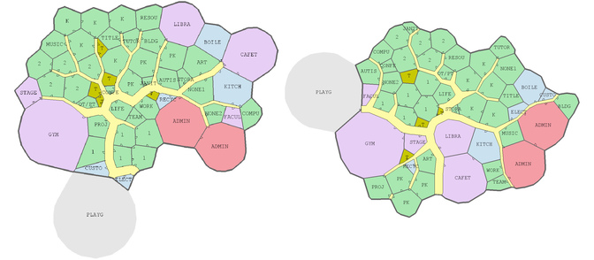
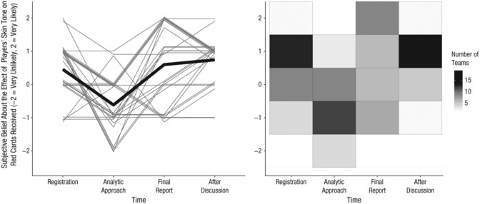
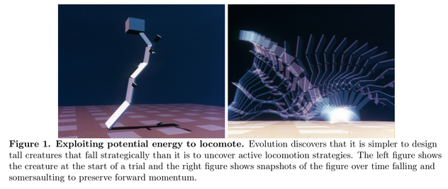

 = \begin{cases}
1 & a_{\mathtt{R}}^t = \mathtt{Invest} \\
0 & a_{\mathtt{R}}^t = \mathtt{Shirk} \\
\end{cases}") .
. &= k + \sum_{t=1}^\infty \delta^t \cdot r^t \cdot k \\
&= k + \frac{\delta \cdot r \cdot k}{1 - \delta \cdot r} \\
U_{\mathtt{P}}(\mathbf{a}) &= (1 - k) - c + \sum_{t=1}^\infty \delta^t \cdot (r ^t \cdot (1 - k) - c) \\
&= (1 - k) - c + \frac{\delta \cdot r \cdot (1 - k)}{1 - \delta \cdot r} - \frac{\delta \cdot c}{1 - \delta} \\
\end{align*}")
 &= l + \sum_{t=1}^\infty \delta^t \cdot r^t \cdot l \\
&= l + \frac{\delta \cdot r \cdot l}{1 - \delta \cdot r} \\
U_{\mathtt{P}}(\mathbf{a}) &= (1 - l) - c + \sum_{t=1}^\infty \delta^t \cdot (r ^t \cdot (1 - l) - c) \\
&= (1 - l) - c + \frac{\delta \cdot r \cdot (1 - l)}{1 - \delta \cdot r} - \frac{\delta \cdot c}{1 - \delta} \\
\end{align*}")
 = (1 - l) - c + \frac{\delta \cdot r \cdot (1 - l)}{1 - \delta \cdot r} - \frac{\delta \cdot c}{1 - \delta} \\
U_{\mathtt{S}}(\mathbf{a}) = (1 - l) + \frac{\delta \cdot (1 - l)}{1 - \delta} \\
(1 - l) - c + \frac{\delta \cdot r \cdot (1 - l)}{1 - \delta \cdot r} - \frac{\delta \cdot c}{1 - \delta} = (1 - l) + \frac{\delta \cdot (1 - l)}{1 - \delta} \\
r = 1 + \frac{c \cdot (1 - \delta)}{c \cdot \delta + \delta \cdot (1 - l)}")
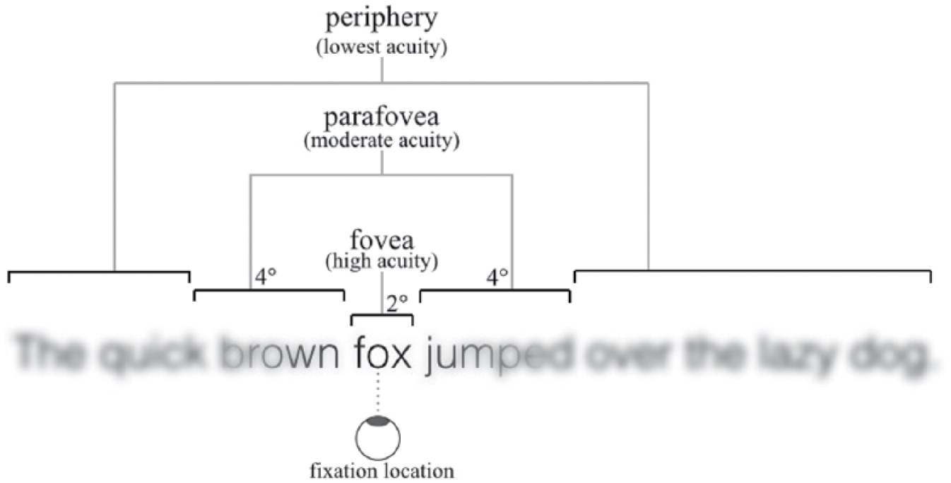
 \\
d_{u} = \text{argmax}_{d \in D} \sum_{\theta \in \Theta} u(\theta, d)")
(1 - D)} &= \frac{KP}{1 - (1 - B)(1 - D)} \\
AS &= KP \\
A(GP - LP) &= KP \\
AP(G - L) &= KP \\
A(G - L) &= K \\
A &= \frac{K}{G - L} \\
A &= \frac{K}{K - 1 + G} \\
\end{align}")
 &= - P(⚀) \log_2 P(⚀) - P(⚁) \log_2 P(⚁) - P(⚂) \log_2 P(⚂) \\
& - P(⚃) \log_2 P(⚃) - P(⚄) \log_2 P(⚄) - P(⚅) \log_2 P(⚅) \\
&= -\left(6 \left(\frac{1}{6} \log_2 \frac{1}{6}\right)\right) \\
&= \log_2 6
\end{align}") .
. &= - P(⚁) \log_2 P(⚁) -
P(⚃) \log_2 P(⚃) -
P(⚅) \log_2 P(⚅) \\
&= - \left(3 \left(\frac{1}{3} \log_2 \frac{1}{3}\right)\right) \\
&= \log_2 3
\end{align}")
 - \cond{H}{A}{\alpha} &= -P(A=t)\log_2P(A=t) - P(A=f)\log_2P(A=f) \\
&+ \cond{P}{A=t}{\alpha}\log_2\cond{P}{A=t}{\alpha} \\
&+ \cond{P}{A=f}{\alpha}\log_2\cond{P}{A=f}{\alpha} \\
&= -0.5\log_20.5 \\
&- 0.5\log_20.5 \\
&+ 0.8\log_20.8 \\
&+ 0.2\log_20.2 \\
&\approx 0.278
\end{align}")


 - \cond{H}{A,B}{\alpha,\beta} &=
\cond{H}{A,B}{\beta} - \cond{H}{A,B}{\alpha,\beta} \\
&+ H(A,B) - \cond{H}{A,B}{\beta}
\end{align}")

 - \cond{H}{A,B,C,D}{\alpha,\beta,\kappa,\delta} &=
\cond{H}{A,B,C,D}{\beta,\kappa,\delta} -
\cond{H}{A,B,C,D}{\alpha,\beta,\kappa,\delta} \\
&+ \cond{H}{A,B,C,D}{\kappa,\delta} -
\cond{H}{A,B,C,D}{\beta,\kappa,\delta} \\
&+ \cond{H}{A,B,C,D}{\delta} - \cond{H}{A,B,C,D}{\kappa,\delta} \\
&+ H(A,B,C,D) - \cond{H}{A,B,C,D}{\delta} \\
\end{align}") leads to scores of
leads to scores of